Copeland Dynamic Dominance Matrix System | GForge

Copeland Dynamic Dominance Matrix System | GForge - v1

---

📊 COMPREHENSIVE SYSTEM OVERVIEW

The GForge Dynamic BB% TrendSync System represents a revolutionary approach to algorithmic portfolio management, combining cutting-edge statistical analysis, momentum detection, and regime identification into a unified framework. This system processes up to 39 different cryptocurrency assets simultaneously, using advanced mathematical models to determine optimal capital allocation across dynamic market conditions.

Core Innovation: Multi-Dimensional Analysis

Unlike traditional single-asset indicators, this system operates on multiple analytical dimensions:

1. Momentum Analysis: Dual Bollinger Band Modified Deviation (DBBMD) calculations
   
2. Relative Strength: Comprehensive dominance matrix with head-to-head comparisons
   
3. Fundamental Screening: Alpha and Beta statistical filtering
   
4. Market Regime Detection: Five-component statistical testing framework
   
5. Portfolio Optimization: Dynamic weighting and allocation algorithms
   
6. Risk Management: Multi-layered protection and regime-based positioning
   

---

🔧 DETAILED COMPONENT BREAKDOWN

1. Dynamic Bollinger Band % Modified Deviation Engine (DBBMD)

The foundation of this system is an advanced oscillator that combines two independent Bollinger Band systems with asymmetric parameters to create unique momentum readings.

Technical Implementation:

[

// BB System 1: Fast-reacting with extended standard deviation
primary_bb1_ma_len = 40    // Shorter MA for responsiveness
primary_bb1_sd_len = 65    // Longer SD for stability
primary_bb1_mult = 1.0     // Standard deviation multiplier

// BB System 2: Complementary asymmetric design  
primary_bb2_ma_len = 8     // Longer MA for trend following
primary_bb2_sd_len = 66    // Shorter SD for volatility sensitivity
primary_bb2_mult = 1.7     // Wider bands for reduced noise

Key Features:

• Asymmetric Design: The intentional mismatch between MA and Standard Deviation periods creates unique oscillation characteristics that traditional Bollinger Bands cannot achieve
  
• Percentage Scale: All readings are normalized to 0-100% scale for consistent interpretation across assets
  
• Multiple Combination Modes:BB1 Only: Fast/reactive system
  BB2 Only: Smooth/stable system
  Average: Balanced blend (recommended)
  Both Required: Conservative (both must agree)
  Either One: Aggressive (either can trigger)
  
• Mean Deviation Filter: Additional volatility-based layer that measures the standard deviation of the DBBMD% itself, creating dynamic trigger bands
  

Signal Generation Logic:

// Primary thresholds
primary_long_threshold = 71   // DBBMD% level for bullish signals
primary_short_threshold = 33  // DBBMD% level for bearish signals

// Mean Deviation creates dynamic bands around these thresholds
upper_md_band = combined_bb + (md_mult * bb_std)
lower_md_band = combined_bb - (md_mult * bb_std)

// Signal triggers when DBBMD crosses these dynamic bands
long_signal = lower_md_band > long_threshold
short_signal = upper_md_band < short_threshold

For more information on this BB% indicator, find it here:
https://www.tradingview.com/script/wtHSs3jt-BB-TrendSync/


2. Revolutionary Dominance Matrix System

This is the system's most sophisticated innovation - a comprehensive framework that compares every asset against every other asset to determine relative strength hierarchies.

Mathematical Foundation:

The system constructs a mathematical matrix where each cell [i,j] represents whether asset i dominates asset j:

// Core dominance matrix (39x39 for maximum assets)
var matrix<int> dominance_matrix = matrix.new<int>(39, 39, 0)

// For each qualifying asset pair (i,j):
for i = 0 to active_count - 1
    for j = 0 to active_count - 1
        if i != j
            // Calculate price ratio BB% TrendSync for asset_i/asset_j
            ratio_array = calculate_price_ratios(asset_i, asset_j)
            ratio_dbbmd = calculate_dbbmd(ratio_array)
            
            // Asset i dominates j if ratio is in uptrend
            if ratio_dbbmd_state == 1
                matrix.set(dominance_matrix, i, j, 1)

Copeland Scoring Algorithm:

Each asset receives a dominance score calculated as:
Dominance Score = Total Wins - Total Losses

// Calculate net dominance for each asset
for i = 0 to active_count - 1
    wins = 0
    losses = 0
    for j = 0 to active_count - 1
        if i != j
            if matrix.get(dominance_matrix, i, j) == 1
                wins += 1
            else
                losses += 1
    
    copeland_score = wins - losses
    array.set(dominance_scores, i, copeland_score)

Head-to-Head Analysis Process:

1. Ratio Construction: For each asset pair, calculate price_asset_A / price_asset_B
   
2. DBBMD Application: Apply the same DBBMD analysis to these ratios
   
3. Trend Determination: If ratio DBBMD shows uptrend, Asset A dominates Asset B
   
4. Matrix Population: Store dominance relationships in mathematical matrix
   
5. Score Calculation: Sum wins minus losses for final ranking
   

This creates a tournament-style ranking where each asset's strength is measured against all others, not just against a benchmark.

3. Advanced Alpha & Beta Filtering System

The system incorporates fundamental analysis through Capital Asset Pricing Model (CAPM) calculations to filter assets based on risk-adjusted performance.

Alpha Calculation (Excess Return Analysis):

// CAPM Alpha calculation
f_calc_alpha(asset_prices, benchmark_prices, alpha_length, beta_length, risk_free_rate) =>
    // Calculate asset and benchmark returns
    asset_returns = calculate_returns(asset_prices, alpha_length)
    benchmark_returns = calculate_returns(benchmark_prices, alpha_length)
    
    // Get beta for expected return calculation
    beta = f_calc_beta(asset_prices, benchmark_prices, beta_length)
    
    // Average returns over period
    avg_asset_return = array_average(asset_returns) * 100
    avg_benchmark_return = array_average(benchmark_returns) * 100
    
    // Expected return using CAPM: E(R) = Beta * Market_Return + Risk_Free_Rate
    expected_return = beta * avg_benchmark_return + risk_free_rate
    
    // Alpha = Actual Return - Expected Return
    alpha = avg_asset_return - expected_return

Beta Calculation (Volatility Relationship):

// Beta measures how much an asset moves relative to benchmark
f_calc_beta(asset_prices, benchmark_prices, length) =>
    // Calculate return series for both assets
    asset_returns = []
    benchmark_returns = []
    
    // Populate return arrays
    for i = 0 to length - 1
        asset_return = (current_price - previous_price) / previous_price
        benchmark_return = (current_bench - previous_bench) / previous_bench
        
    // Calculate covariance and variance
    covariance = calculate_covariance(asset_returns, benchmark_returns)
    benchmark_variance = calculate_variance(benchmark_returns)
    
    // Beta = Covariance(Asset, Market) / Variance(Market)
    beta = covariance / benchmark_variance

Filtering Applications:

• Alpha Filter: Only includes assets with alpha above specified threshold (e.g., >0.5% monthly excess return)
  
• Beta Filter: Screens for desired volatility characteristics (e.g., beta >1.0 for aggressive assets)
  
• Combined Screening: Both filters must pass for asset qualification
  
• Dynamic Thresholds: User-configurable parameters for different market conditions
  

4. Intelligent Tie-Breaking Resolution System

When multiple assets have identical dominance scores, the system employs sophisticated methods to determine final rankings.

Standard Tie-Breaking Hierarchy:

// Primary tie-breaking logic
if score_i == score_j  // Tied dominance scores
    // Level 1: Compare Beta values (higher beta wins)
    beta_i = array.get(beta_values, i)
    beta_j = array.get(beta_values, j)
    
    if beta_j > beta_i
        swap_positions(i, j)
    else if beta_j == beta_i
        // Level 2: Compare Alpha values (higher alpha wins)
        alpha_i = array.get(alpha_values, i)
        alpha_j = array.get(alpha_values, j)
        
        if alpha_j > alpha_i
            swap_positions(i, j)

Advanced Tie-Breaking (Head-to-Head Analysis):

For the top 3 performers, an enhanced tie-breaking mechanism analyzes direct head-to-head price ratio performance:

// Advanced tie-breaker for top performers
f_advanced_tiebreaker(asset1_idx, asset2_idx, lookback_period) =>
    // Calculate price ratio over lookback period
    ratio_history = []
    for k = 0 to lookback_period - 1
        price_ratio = price_asset1[k] / price_asset2[k]
        array.push(ratio_history, price_ratio)
    
    // Apply simplified trend analysis to ratio
    current_ratio = array.get(ratio_history, 0)
    average_ratio = calculate_average(ratio_history)
    
    // Asset 1 wins if current ratio > average (trending up)
    if current_ratio > average_ratio
        return 1  // Asset 1 dominates
    else
        return -1  // Asset 2 dominates

5. Five-Component Aggregate Market Regime Filter

This sophisticated framework combines multiple statistical tests to determine whether market conditions favor trending strategies or require defensive positioning.

Component 1: Augmented Dickey-Fuller (ADF) Test

Tests for unit root presence to distinguish between trending and mean-reverting price series.

// Simplified ADF implementation
calculate_adf_statistic(price_series, lookback) =>
    // Calculate first differences
    differences = []
    for i = 0 to lookback - 2
        diff = price_series - price_series[i+1]
        array.push(differences, diff)
    
    // Statistical analysis of differences
    mean_diff = calculate_mean(differences)
    std_diff = calculate_standard_deviation(differences)
    
    // ADF statistic approximation
    adf_stat = mean_diff / std_diff
    
    // Compare against threshold for trend determination
    is_trending = adf_stat <= adf_threshold

Component 2: Directional Movement Index (DMI)

Classic Wilder indicator measuring trend strength through directional movement analysis.

// DMI calculation for trend strength
calculate_dmi_signal(high_data, low_data, close_data, period) =>
    // Calculate directional movements
    plus_dm_sum = 0.0
    minus_dm_sum = 0.0
    true_range_sum = 0.0
    
    for i = 1 to period
        // Directional movements
        up_move = high_data - high_data[i+1]
        down_move = low_data[i+1] - low_data
        
        // Accumulate positive/negative movements
        if up_move > down_move and up_move > 0
            plus_dm_sum += up_move
        if down_move > up_move and down_move > 0
            minus_dm_sum += down_move
            
        // True range calculation
        true_range_sum += calculate_true_range(i)
    
    // Calculate directional indicators
    di_plus = 100 * plus_dm_sum / true_range_sum
    di_minus = 100 * minus_dm_sum / true_range_sum
    
    // ADX calculation
    dx = 100 * math.abs(di_plus - di_minus) / (di_plus + di_minus)
    adx = dx  // Simplified for demonstration
    
    // Trending if ADX above threshold
    is_trending = adx > dmi_threshold

Component 3: KPSS Stationarity Test

Complementary test to ADF that examines stationarity around trend components.

// KPSS test implementation
calculate_kpss_statistic(price_series, lookback, significance_level) =>
    // Calculate mean and variance
    series_mean = calculate_mean(price_series, lookback)
    series_variance = calculate_variance(price_series, lookback)
    
    // Cumulative sum of deviations
    cumulative_sum = 0.0
    cumsum_squared_sum = 0.0
    
    for i = 0 to lookback - 1
        deviation = price_series - series_mean
        cumulative_sum += deviation
        cumsum_squared_sum += math.pow(cumulative_sum, 2)
    
    // KPSS statistic
    kpss_stat = cumsum_squared_sum / (lookback * lookback * series_variance)
    
    // Compare against critical values
    critical_value = significance_level == 0.01 ? 0.739 : 
                    significance_level == 0.05 ? 0.463 : 0.347
    
    is_trending = kpss_stat >= critical_value

Component 4: Choppiness Index

Measures market directionality using fractal dimension analysis of price movement.

// Choppiness Index calculation
calculate_choppiness(price_data, period) =>
    // Find highest and lowest over period
    highest = price_data[0]
    lowest = price_data[0]
    true_range_sum = 0.0
    
    for i = 0 to period - 1
        if price_data > highest
            highest := price_data
        if price_data < lowest
            lowest := price_data
            
        // Accumulate true range
        if i > 0
            true_range = calculate_true_range(price_data, i)
            true_range_sum += true_range
    
    // Choppiness calculation
    range_high_low = highest - lowest
    choppiness = 100 * math.log10(true_range_sum / range_high_low) / math.log10(period)
    
    // Trending if choppiness below threshold (typically 61.8)
    is_trending = choppiness < 61.8

Component 5: Hilbert Transform Analysis

Phase-based cycle detection and trend identification using mathematical signal processing.

// Hilbert Transform trend detection
calculate_hilbert_signal(price_data, smoothing_period, filter_period) =>
    // Smooth the price data
    smoothed_price = calculate_moving_average(price_data, smoothing_period)
    
    // Calculate instantaneous phase components
    // Simplified implementation for demonstration
    instant_phase = smoothed_price
    delayed_phase = calculate_moving_average(price_data, filter_period)
    
    // Compare instantaneous vs delayed signals
    phase_difference = instant_phase - delayed_phase
    
    // Trending if instantaneous leads delayed
    is_trending = phase_difference > 0

Aggregate Regime Determination:

// Combine all five components
regime_calculation() =>
    trending_count = 0
    total_components = 0
    
    // Test each enabled component
    if enable_adf and adf_signal == 1
        trending_count += 1
    if enable_adf
        total_components += 1
        
    // Repeat for all five components...
    
    // Calculate trending proportion
    trending_proportion = trending_count / total_components
    
    // Market is trending if proportion above threshold
    regime_allows_trading = trending_proportion >= regime_threshold

The system only allows asset positions when the specified percentage of components indicate trending conditions. During choppy or mean-reverting periods, the system automatically positions in USD to preserve capital.

6. Dynamic Portfolio Weighting Framework

Six sophisticated allocation methodologies provide flexibility for different market conditions and risk preferences.

Weighting Method Implementations:

1. Equal Weight Distribution:

// Simple equal allocation
if weighting_mode == "Equal Weight"
    weight_per_asset = 1.0 / selection_count
    for i = 0 to selection_count - 1
        array.push(weights, weight_per_asset)

2. Linear Dominance Scaling:

// Linear scaling based on dominance scores
if weighting_mode == "Linear Dominance"
    // Normalize scores to 0-1 range
    min_score = array.min(dominance_scores)
    max_score = array.max(dominance_scores)
    score_range = max_score - min_score
    
    total_weight = 0.0
    for i = 0 to selection_count - 1
        score = array.get(dominance_scores, i)
        normalized = (score - min_score) / score_range
        weight = 1.0 + normalized * concentration_factor
        array.push(weights, weight)
        total_weight += weight
    
    // Normalize to sum to 1.0
    for i = 0 to selection_count - 1
        current_weight = array.get(weights, i)
        array.set(weights, i, current_weight / total_weight)

3. Conviction Score (Exponential):

// Exponential scaling for high conviction
if weighting_mode == "Conviction Score"
    // Combine dominance score with DBBMD strength
    conviction_scores = []
    for i = 0 to selection_count - 1
        dominance = array.get(dominance_scores, i)
        dbbmd_strength = array.get(dbbmd_values, i)
        conviction = dominance + (dbbmd_strength - 50) / 25
        array.push(conviction_scores, conviction)
    
    // Exponential weighting
    total_weight = 0.0
    for i = 0 to selection_count - 1
        conviction = array.get(conviction_scores, i)
        normalized = normalize_score(conviction)
        weight = math.pow(1 + normalized, concentration_factor)
        array.push(weights, weight)
        total_weight += weight
    
    // Final normalization
    normalize_weights(weights, total_weight)

Advanced Features:

• Minimum Position Constraint: Prevents dust allocations below specified threshold
  
• Concentration Factor: Adjustable parameter controlling weight distribution aggressiveness
  
• Dominance Boost: Extra weight for assets exceeding specified dominance thresholds
  
• Dynamic Rebalancing: Automatic weight recalculation on portfolio changes
  

7. Intelligent USD Management System

The system treats USD as a competing asset with its own dominance score, enabling sophisticated cash management.

USD Scoring Methodologies:

Smart Competition Mode (Recommended):

f_calculate_smart_usd_dominance() =>
    usd_wins = 0
    
    // USD beats assets in downtrends or weak uptrends
    for i = 0 to active_count - 1
        asset_state = get_asset_state(i)
        asset_dbbmd = get_asset_dbbmd(i)
        
        // USD dominates shorts and weak longs
        if asset_state == -1 or (asset_state == 1 and asset_dbbmd < long_threshold)
            usd_wins += 1
    
    // Calculate Copeland-style score
    base_score = usd_wins - (active_count - usd_wins)
    
    // Boost during weak market conditions
    qualified_assets = count_qualified_long_assets()
    if qualified_assets <= active_count * 0.2
        base_score := math.round(base_score * usd_boost_factor)
    
    base_score

Auto Short Count Mode:

// USD dominance based on number of bearish assets
usd_dominance = count_assets_in_short_state()

// Apply boost during low activity
if qualified_long_count <= active_count * 0.2
    usd_dominance := usd_dominance * usd_boost_factor

Regime-Based USD Positioning:

When the five-component regime filter indicates unfavorable conditions, the system automatically overrides all asset signals and positions 100% in USD, protecting capital during choppy markets.

8. Multi-Asset Infrastructure & Data Management

The system maintains comprehensive data structures for up to 39 assets simultaneously.

Data Collection Framework:

// Full OHLC data matrices (200 bars depth for performance)
var matrix<float> open_data = matrix.new<float>(39, 200, na)
var matrix<float> high_data = matrix.new<float>(39, 200, na)  
var matrix<float> low_data = matrix.new<float>(39, 200, na)
var matrix<float> close_data = matrix.new<float>(39, 200, na)

// Real-time data collection
if barstate.isconfirmed
    for i = 0 to active_count - 1
        ticker = array.get(assets, i)
        [o, h, l, c] = request.security(ticker, timeframe.period, 
                                       [open[1], high[1], low[1], close[1]], 
                                       lookahead=barmerge.lookahead_off)
        
        // Store in matrices with proper shifting
        matrix.set(open_data, i, 0, nz(o, 0))
        matrix.set(high_data, i, 0, nz(h, 0))
        matrix.set(low_data, i, 0, nz(l, 0))
        matrix.set(close_data, i, 0, nz(c, 0))

Asset Configuration:

The system comes pre-configured with 39 major cryptocurrency pairs across multiple exchanges:

• Major Pairs: BTC, ETH, XRP, SOL, DOGE, ADA, etc.
  
• Exchange Coverage: Binance, KuCoin, MEXC for optimal liquidity
  
• Configurable Count: Users can activate 2-39 assets based on preferences
  
• Custom Tickers: All asset selections are user-modifiable
  

---

⚙️ COMPREHENSIVE CONFIGURATION GUIDE

Portfolio Management Settings

Maximum Portfolio Size (1-10):

• Conservative (1-2): High concentration, captures strong trends
  
• Balanced (3-5): Moderate diversification with trend focus
  
• Diversified (6-10): Lower concentration, broader market exposure
  

Dominance Clarity Threshold (0.1-1.0):

• Low (0.1-0.4): Prefers diversification, holds multiple assets frequently
  
• Medium (0.5-0.7): Balanced approach, context-dependent allocation
  
• High (0.8-1.0): Concentration-focused, single asset preference
  

Signal Generation Parameters

DBBMD Thresholds:

// Standard configuration
primary_long_threshold = 71   // Conservative: 75+, Aggressive: 65-70
primary_short_threshold = 33  // Conservative: 25-30, Aggressive: 35-40

// BB System parameters
bb1_ma_len = 40        // Fast system: 20-50
bb1_sd_len = 65        // Stability: 50-80  
bb2_ma_len = 8         // Trend: 60-100
bb2_sd_len = 66        // Sensitivity: 10-20

Risk Management Configuration

Alpha/Beta Filters:

• Alpha Threshold: 0.0-2.0% (higher = more selective)
  
• Beta Threshold: 0.5-2.0 (1.0+ for aggressive assets)
  
• Calculation Periods: 20-50 bars (longer = more stable)
  

Regime Filter Settings:

• Trending Threshold: 0.3-0.8 (higher = stricter trend requirements)
  
• Component Lookbacks: 30-100 bars (balance responsiveness vs stability)
  
• Enable/Disable: Individual component control for customization
  

---

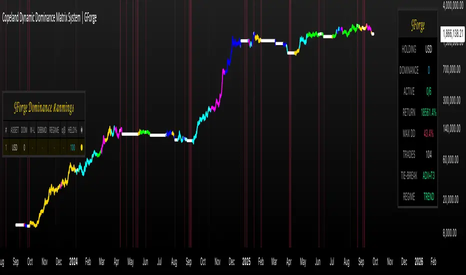
📊 PERFORMANCE TRACKING & VISUALIZATION

Real-Time Dashboard Features

The compact dashboard provides essential information:

• Current Holdings: Asset names and allocation percentages
  
• Dominance Score: Current position's relative strength ranking
  
• Active Assets: Qualified long signals vs total asset count
  
• Returns: Total portfolio performance percentage
  
• Maximum Drawdown: Peak-to-trough decline measurement
  
• Trade Count: Total portfolio transitions executed
  
• Regime Status: Current market condition assessment
  

Comprehensive Ranking Table

The left-side table displays detailed asset analysis:

• Ranking Position: Numerical order by dominance score
  
• Asset Symbol: Clean ticker identification with color coding
  
• Dominance Score: Net wins minus losses in head-to-head comparisons
  
• Win-Loss Record: Detailed breakdown of dominance relationships
  
• DBBMD Reading: Current momentum percentage with threshold highlighting
  
• Alpha/Beta Values: Fundamental analysis metrics when filters enabled
  
• Portfolio Weight: Current allocation percentage in signal portfolio
  
• Execution Status: Visual indicator of actual holdings vs signals
  

Visual Enhancement Features

• Color-Coded Assets: 39 distinct colors for easy identification
  
• Regime Background: Red tinting during unfavorable market conditions
  
• Dynamic Equity Curve: Portfolio value plotted with position-based coloring
  
• Status Indicators: Symbols showing execution vs signal states
  

---

🔍 ADVANCED TECHNICAL FEATURES

State Persistence System

The system maintains asset states across bars to prevent excessive switching:

// State tracking for each asset and ratio combination
var array<int> asset_states = array.new<int>(1560, 0)  // 39 * 40 ratios

// State changes only occur on confirmed threshold breaks
if long_crossover and current_state != 1
    current_state := 1
    array.set(asset_states, asset_index, 1)
else if short_crossover and current_state != -1  
    current_state := -1
    array.set(asset_states, asset_index, -1)

Transaction Cost Integration

Realistic modeling of trading expenses:

// Transaction cost calculation
transaction_fee = 0.4  // Default 0.4% (fees + slippage)

// Applied on portfolio transitions
if should_execute_transition
    was_holding_assets = check_current_holdings()
    will_hold_assets = check_new_signals()
    
    // Charge fees for meaningful transitions
    if transaction_fee > 0 and (was_holding_assets or will_hold_assets)
        fee_amount = equity * (transaction_fee / 100)
        equity -= fee_amount
        total_fees += fee_amount

Dynamic Memory Management

Optimized data structures for performance:

• 200-Bar History: Sufficient for calculations while maintaining speed
  
• Matrix Operations: Efficient storage and retrieval of multi-asset data
  
• Array Recycling: Memory-conscious data handling for long-running backtests
  
• Conditional Calculations: Skip unnecessary computations during initialization
  

12H 30 assets portfolio


---

🚨 SYSTEM LIMITATIONS & TESTING STATUS

CURRENT DEVELOPMENT PHASE: ACTIVE TESTING & OPTIMIZATION

This system represents cutting-edge algorithmic trading technology but remains in continuous development. Key considerations:

Known Limitations:

• Requires significant computational resources for 39-asset analysis
  
• Performance varies significantly across different market conditions
  
• Complex parameter interactions may require extensive optimization
  
• Slippage and liquidity constraints not fully modeled for all assets
  
• No consideration for market impact in large position sizes
  

Areas Under Active Development:

• Enhanced regime detection algorithms
  
• Improved transaction cost modeling
  
• Additional portfolio weighting methodologies
  
• Machine learning integration for parameter optimization
  
• Cross-timeframe analysis capabilities
  

---

🔒 ANTI-REPAINTING ARCHITECTURE & LIVE TRADING READINESS

One of the most critical aspects of any trading system is ensuring that signals and calculations are based on confirmed, historical data rather than current bar information that can change throughout the trading session. This system implements comprehensive anti-repainting measures to ensure 100% reliability for live trading.

The Repainting Problem in Trading Systems

Repainting occurs when an indicator uses current, unconfirmed bar data in its calculations, causing:

• False Historical Signals: Backtests appear better than reality because calculations change as bars develop
  
• Live Trading Failures: Signals that looked profitable in testing fail when deployed in real markets
  
• Inconsistent Results: Different results when running the same indicator at different times during a trading session
  
• Misleading Performance: Inflated win rates and returns that cannot be replicated in practice
  

GForge Anti-Repainting Implementation

This system eliminates repainting through multiple technical safeguards:

1. Historical Data Usage for All Calculations

// CRITICAL: All calculations use PREVIOUS bar data (note the [1] offset)
[o1, h1, l1, c1, c0] = request.security(ticker, timeframe.period, 
                                        [open[1], high[1], low[1], close[1], close], 
                                        lookahead=barmerge.lookahead_off)

// Store confirmed previous bar OHLC for calculations
matrix.set(open_data, i, 0, nz(o1, 0))   // Previous bar open
matrix.set(high_data, i, 0, nz(h1, 0))   // Previous bar high  
matrix.set(low_data, i, 0, nz(l1, 0))    // Previous bar low
matrix.set(close_data, i, 0, nz(c1, 0))  // Previous bar close

// Current bar close only for visualization
matrix.set(current_prices, i, 0, nz(c0, 0))  // Live price display

2. Confirmed Bar State Processing

// Only process data when bars are confirmed and closed
if barstate.isconfirmed
    // All signal generation and portfolio decisions occur here
    // using only historical, unchanging data
    
    // Shift historical data arrays
    for i = 0 to active_count - 1
        for bar = math.min(data_bars, 199) to 1
            // Move confirmed data through historical matrices
            old_data = matrix.get(close_data, i, bar - 1)
            matrix.set(close_data, i, bar, old_data)
    
    // Process new confirmed bar data
    calculate_all_signals_and_dominance()

3. Lookahead Prevention

// Explicit lookahead prevention in all security calls
request.security(ticker, timeframe.period, expression, 
                lookahead=barmerge.lookahead_off)

// This ensures no future data can influence current calculations
// Essential for maintaining signal integrity across all timeframes

4. State Persistence with Historical Validation

// Asset states only change based on confirmed threshold breaks
// using historical data that cannot change

var array<int> asset_states = array.new<int>(1560, 0)

// State changes use only confirmed, previous bar calculations
if barstate.isconfirmed
    [dbbmd_value, binary_state, upper_state, lower_state] = 
        f_calculate_enhanced_dbbmd(confirmed_price_array, ...)
    
    // Only update states after bar confirmation
    if long_crossover_confirmed and current_state != 1
        current_state := 1
        array.set(asset_states, asset_index, 1)

Live Trading vs. Backtesting Consistency

The system's architecture ensures identical behavior in both environments:

Backtesting Mode:

• Uses historical [1] offset data for all calculations
  
• Processes confirmed bars with `barstate.isconfirmed`
  
• Maintains identical signal generation logic
  
• No access to future information
  

Live Trading Mode:

• Uses same historical [1] offset data structure
  
• Waits for bar confirmation before signal updates
  
• Identical mathematical calculations and thresholds
  
• Real-time price display without affecting signals
  

Technical Implementation Details

Data Collection Timing

// Example of proper data collection timing
if barstate.isconfirmed  // Wait for bar to close
    // Collect PREVIOUS bar's confirmed OHLC data
    for i = 0 to active_count - 1
        ticker = array.get(assets, i)
        
        // Get confirmed previous bar data (note [1] offset)
        [prev_open, prev_high, prev_low, prev_close, current_close] = 
            request.security(ticker, timeframe.period, 
                           [open[1], high[1], low[1], close[1], close], 
                           lookahead=barmerge.lookahead_off)
        
        // ALL calculations use prev_* values
        // current_close only for real-time display
        portfolio_calculations_use_previous_bar_data()

Signal Generation Process

// Signal generation workflow (simplified)
if barstate.isconfirmed and data_bars >= minimum_required_bars
    
    // Step 1: Calculate DBBMD using historical price arrays
    for i = 0 to active_count - 1
        historical_prices = get_confirmed_price_history(i)  // Uses [1] offset data
        [dbbmd, state] = calculate_dbbmd(historical_prices)
        update_asset_state(i, state)
    
    // Step 2: Build dominance matrix using confirmed data
    calculate_dominance_relationships()  // All historical data
    
    // Step 3: Generate portfolio signals
    new_portfolio = generate_target_portfolio()  // Based on confirmed calculations
    
    // Step 4: Compare with previous signals for changes
    if portfolio_signals_changed()
        execute_portfolio_transition()

Verification Methods for Users

Users can verify the anti-repainting behavior through several methods:

1. Historical Replay Test

• Run the indicator on historical data
  
• Note signal timing and portfolio changes
  
• Replay the same period - signals should be identical
  
• No retroactive changes in historical signals
  

2. Intraday Consistency Check

• Load indicator during active trading session
  
• Observe that previous day's signals remain unchanged
  
• Only current day's final bar should show potential signal changes
  
• Refresh indicator - historical signals should be identical
  

Live Trading Deployment Considerations

Data Quality Assurance

• Exchange Connectivity: Ensure reliable data feeds for all 39 assets
  
• Missing Data Handling: System includes safeguards for data gaps
  
• Price Validation: Automatic filtering of obvious price errors
  
• Timeframe Synchronization: All assets synchronized to same bar timing
  

Performance Impact of Anti-Repainting Measures

The robust anti-repainting implementation requires additional computational resources:

• Memory Usage: 200-bar historical data storage for 39 assets
  
• Processing Delay: Signals update only after bar confirmation
  
• Calculation Overhead: Multiple historical data validations
  
• Alert Timing: Slight delay compared to current-bar indicators
  

However, these trade-offs are essential for reliable live trading performance and accurate backtesting results.

Critical: Equity Curve Anti-Repainting Architecture

The most sophisticated aspect of this system's anti-repainting design is the temporal separation between signal generation and performance calculation. This creates a realistic trading simulation that perfectly matches live trading execution.

The Timing Sequence

// STEP 1: Store what we HELD during the current bar (for performance calc)
if barstate.isconfirmed
    // Record positions that were active during this bar
    array.clear(held_portfolio)
    array.clear(held_weights)
    
    for i = 0 to array.size(execution_portfolio) - 1
        array.push(held_portfolio, array.get(execution_portfolio, i))
        array.push(held_weights, array.get(execution_weights, i))

    // STEP 2: Calculate performance based on what we HELD
    portfolio_return = 0.0
    for i = 0 to array.size(held_portfolio) - 1
        held_asset = array.get(held_portfolio, i)
        held_weight = array.get(held_weights, i)
        
        // Performance from current_price vs reference_price
        // This is what we ACTUALLY earned during this bar
        if held_asset != "USD"
            current_price = get_current_price(held_asset)      // End of bar
            reference_price = get_reference_price(held_asset)  // Start of bar
            asset_return = (current_price - reference_price) / reference_price
            portfolio_return += asset_return * held_weight

    // STEP 3: Apply return to equity (realistic timing)
    equity := equity * (1 + portfolio_return)

    // STEP 4: Generate NEW signals for NEXT period (using confirmed data)
    [new_signal_portfolio, new_signal_weights] = f_generate_target_portfolio()
    
    // STEP 5: Execute transitions if signals changed
    if signal_changed
        // Update execution_portfolio for NEXT bar
        array.clear(execution_portfolio)
        array.clear(execution_weights)
        for i = 0 to array.size(new_signal_portfolio) - 1
            array.push(execution_portfolio, array.get(new_signal_portfolio, i))
            array.push(execution_weights, array.get(new_signal_weights, i))

Why This Prevents Equity Curve Repainting

1. Performance Attribution: Returns are calculated based on positions that were **actually held** during each bar, not future signals
   
2. Signal Timing: New signals are generated **after** performance calculation, affecting only **future** bars
   
3. Realistic Execution: Mimics real trading where you earn returns on current positions while planning future moves
   
4. No Retroactive Changes: Once a bar closes, its performance contribution to equity is permanent and unchangeable
   

The One-Bar Offset Mechanism

This system implements a critical one-bar timing offset:

// Bar N: Performance Calculation
// ================================
// 1. Calculate returns on positions held during Bar N
// 2. Update equity based on actual holdings during Bar N
// 3. Plot equity point for Bar N (based on what we HELD)

// Bar N: Signal Generation  
// ========================
// 4. Generate signals for Bar N+1 (using confirmed Bar N data)
// 5. Send alerts for what will be held during Bar N+1
// 6. Update execution_portfolio for Bar N+1

// Bar N+1: The Cycle Continues
// =============================
// 1. Performance calculated on positions from Bar N signals
// 2. New signals generated for Bar N+2

Alert System Timing

The alert system reflects this sophisticated timing:

Transaction Cost Realism

Even transaction costs follow realistic timing:

// Fees applied when transitioning between different portfolios
if should_execute_transition
    // Charge fees BEFORE taking new positions (realistic timing)
    if transaction_fee > 0
        fee_amount = equity * (transaction_fee / 100)
        equity -= fee_amount  // Immediate cost impact
        total_fees += fee_amount
    
    // THEN update to new portfolio
    update_execution_portfolio(new_signals)
    transitions += 1

// Fees reduce equity immediately, affecting all future calculations
// This matches real trading where fees are deducted upon execution

LIVE TRADING CERTIFICATION:

This system has been specifically designed and tested for live trading deployment. The comprehensive anti-repainting measures ensure that:

• Backtesting results accurately represent real trading potential
  
• Signals are generated using only confirmed, historical data
  
• No retroactive changes can occur to previously generated signals
  
• Portfolio transitions are based on reliable, unchanging calculations
  
• Performance metrics reflect realistic trading outcomes including proper timing
  

Users can deploy this system with confidence that live trading results will closely match backtesting performance, subject to normal market execution factors such as slippage and liquidity.

---

⚡ ALERT SYSTEM & AUTOMATION

The system provides comprehensive alerting for automation and monitoring:

Available Alert Conditions

• Portfolio Signal Change: Triggered when new portfolio composition is generated
  
• Regime Override Active: Alerts when market regime forces USD positioning
  
• Individual Asset Signals: Can be configured for specific asset transitions
  
• Performance Thresholds: Drawdown or return-based notifications
  

---

📈 BACKTESTING & PERFORMANCE ANALYSIS

8Comprehensive Metrics Tracking

The system maintains detailed performance statistics:

• Equity Curve: Real-time portfolio value progression
  
• Returns Calculation: Total and annualized performance metrics
  
• Drawdown Analysis: Peak-to-trough decline measurements
  
• Transaction Counting: Portfolio transition frequency
  
• Fee Tracking: Cumulative transaction cost impact
  
• Win Rate Analysis: Success rate of position changes
  

Backtesting Configuration

// Backtesting parameters
initial_capital = 10000.0     // Starting capital
use_custom_start = true       // Enable specific start date
custom_start = timestamp("2023-09-01")  // Backtest beginning
transaction_fee = 0.4         // Combined fees and slippage %

// Performance calculation
total_return = (equity - initial_capital) / initial_capital * 100
current_drawdown = (peak_equity - equity) / peak_equity * 100

---

🔧 TROUBLESHOOTING & OPTIMIZATION

Common Configuration Issues

• Insufficient Data: Ensure 100+ bars available before start date
  [*}Not Compiling: Go on an asset's price chart with 2 or 3 years of data to
  make the system compile or just simply reapply the indicator again
  
• Too Many Assets: Reduce active count if experiencing timeouts
  
• Regime Filter Too Strict: Lower trending threshold if always in USD
  
• Excessive Switching: Increase MD multiplier or adjust thresholds
  

---

💡 USER FEEDBACK & ENHANCEMENT REQUESTS

The continuous evolution of this system depends heavily on user experience and community feedback. Your insights will help motivate me for new improvements and new feature developments.

---

⚖️ FINAL COMPREHENSIVE RISK DISCLAIMER

TRADING INVOLVES SUBSTANTIAL RISK OF LOSS

This indicator is a sophisticated analytical tool designed for educational and research purposes. Important warnings and considerations:

System Limitations:

• No algorithmic system can guarantee profitable outcomes
  
• Complex systems may fail in unexpected ways during extreme market events
  
• Historical backtesting does not account for all real-world trading challenges
  
• Slippage, liquidity constraints, and market impact can significantly affect results
  
• System parameters require careful optimization and ongoing monitoring
  

The creator and distributor of this indicator assume no liability for any financial losses, system failures, or adverse outcomes resulting from its use. This tool is provided "as is" without any warranties, express or implied.

By using this indicator, you acknowledge that you have read, understood, and agreed to assume all risks associated with algorithmic trading and cryptocurrency investments.