SuperTrend AI (Clustering) [LuxAlgo]The SuperTrend AI indicator is a novel take on bridging the gap between the K-means clustering machine learning method & technical indicators. In this case, we apply K-Means clustering to the famous SuperTrend indicator.
🔶 USAGE
Users can interpret the SuperTrend AI trailing stop similarly to the regular SuperTrend indicator. Using higher minimum/maximum factors will return longer-term signals.
The displayed performance metrics displayed on each signal allow for a deeper interpretation of the indicator. Whereas higher values could indicate a higher potential for the market to be heading in the direction of the trend when compared to signals with lower values such as 1 or 0 potentially indicating retracements.
In the image above, we can notice more clear examples of the performance metrics on signals indicating trends, however, these performance metrics cannot perform or predict every signal reliably.
We can see in the image above that the trailing stop and its adaptive moving average can also act as support & resistance. Using higher values of the performance memory setting allows users to obtain a longer-term adaptive moving average of the returned trailing stop.
🔶 DETAILS
🔹 K-Means Clustering
When observing data points within a specific space, we can sometimes observe that some are closer to each other, forming groups, or "Clusters". At first sight, identifying those clusters and finding their associated data points can seem easy but doing so mathematically can be more challenging. This is where cluster analysis comes into play, where we seek to group data points into various clusters such that data points within one cluster are closer to each other. This is a common branch of AI/machine learning.
Various methods exist to find clusters within data, with the one used in this script being K-Means Clustering , a simple iterative unsupervised clustering method that finds a user-set amount of clusters.
A naive form of the K-Means algorithm would perform the following steps in order to find K clusters:
(1) Determine the amount (K) of clusters to detect.
(2) Initiate our K centroids (cluster centers) with random values.
(3) Loop over the data points, and determine which is the closest centroid from each data point, then associate that data point with the centroid.
(4) Update centroids by taking the average of the data points associated with a specific centroid.
Repeat steps 3 to 4 until convergence, that is until the centroids no longer change.
To explain how K-Means works graphically let's take the example of a one-dimensional dataset (which is the dimension used in our script) with two apparent clusters:
This is of course a simple scenario, as K will generally be higher, as well the amount of data points. Do note that this method can be very sensitive to the initialization of the centroids, this is why it is generally run multiple times, keeping the run returning the best centroids.
🔹 Adaptive SuperTrend Factor Using K-Means
The proposed indicator rationale is based on the following hypothesis:
Given multiple instances of an indicator using different settings, the optimal setting choice at time t is given by the best-performing instance with setting s(t) .
Performing the calculation of the indicator using the best setting at time t would return an indicator whose characteristics adapt based on its performance. However, what if the setting of the best-performing instance and second best-performing instance of the indicator have a high degree of disparity without a high difference in performance?
Even though this specific case is rare its however not uncommon to see that performance can be similar for a group of specific settings (this could be observed in a parameter optimization heatmap), then filtering out desirable settings to only use the best-performing one can seem too strict. We can as such reformulate our first hypothesis:
Given multiple instances of an indicator using different settings, an optimal setting choice at time t is given by the average of the best-performing instances with settings s(t) .
Finding this group of best-performing instances could be done using the previously described K-Means clustering method, assuming three groups of interest (K = 3) defined as worst performing, average performing, and best performing.
We first obtain an analog of performance P(t, factor) described as:
P(t, factor) = P(t-1, factor) + α * (∆C(t) × S(t-1, factor) - P(t-1, factor))
where 1 > α > 0, which is the performance memory determining the degree to which older inputs affect the current output. C(t) is the closing price, and S(t, factor) is the SuperTrend signal generating function with multiplicative factor factor .
We run this performance function for multiple factor settings and perform K-Means clustering on the multiple obtained performances to obtain the best-performing cluster. We initiate our centroids using quartiles of the obtained performances for faster centroids convergence.
The average of the factors associated with the best-performing cluster is then used to obtain the final factor setting, which is used to compute the final SuperTrend output.
Do note that we give the liberty for the user to get the final factor from the best, average, or worst cluster for experimental purposes.
🔶 SETTINGS
ATR Length: ATR period used for the calculation of the SuperTrends.
Factor Range: Determine the minimum and maximum factor values for the calculation of the SuperTrends.
Step: Increments of the factor range.
Performance Memory: Determine the degree to which older inputs affect the current output, with higher values returning longer-term performance measurements.
From Cluster: Determine which cluster is used to obtain the final factor.
🔹 Optimization
This group of settings affects the runtime performances of the script.
Maximum Iteration Steps: Maximum number of iterations allowed for finding centroids. Excessively low values can return a better script load time but poor clustering.
Historical Bars Calculation: Calculation window of the script (in bars).
Machinelearning

Machine Learning Momentum Index (MLMI) [Zeiierman]█ Overview
The Machine Learning Momentum Index (MLMI) represents the next step in oscillator trading. By blending traditional momentum analysis with machine learning, MLMI delivers a potent and dynamic tool that aligns with the complexities of modern financial landscapes. Offering traders an adaptive way to understand and act on market momentum and trends, this oscillator provides real-time insights into market momentum and prevailing trends.
█ How It Works:
Momentum Analysis: MLMI employs a dual-layer analysis, utilizing quick and slow weighted moving averages (WMA) of the Relative Strength Index (RSI) to gauge the market's momentum and direction.
Machine Learning Integration: Through the k-Nearest Neighbors (k-NN) algorithm, MLMI intelligently examines historical data to make more accurate momentum predictions, adapting to the intricate patterns of the market.
MLMI's precise calculation involves:
Weighted Moving Averages: Calculations of quick (5-period) and slow (20-period) WMAs of the RSI to track short-term and long-term momentum.
k-Nearest Neighbors Algorithm: Distances between current parameters and previous data are measured, and the nearest neighbors are used for predictive modeling.
Trend Analysis: Recognition of prevailing trends through the relationship between quick and slow-moving averages.
█ How to use
The Machine Learning Momentum Index (MLMI) can be utilized in much the same way as traditional trend and momentum oscillators, providing key insights into market direction and strength. What sets MLMI apart is its integration of artificial intelligence, allowing it to adapt dynamically to market changes and offer a more nuanced and responsive analysis.
Identifying Trend Direction and Strength: The MLMI serves as a tool to recognize market trends, signaling whether the momentum is upward or downward. It also provides insights into the intensity of the momentum, helping traders understand both the direction and strength of prevailing market trends.
Identifying Consolidation Areas: When the MLMI Prediction line and the WMA of the MLMI Prediction line become flat/oscillate around the mid-level, it's a strong sign that the market is in a consolidation phase. This insight from the MLMI allows traders to recognize periods of market indecision.
Recognizing Overbought or Oversold Conditions: By identifying levels where the market may be overbought or oversold, MLMI offers insights into potential price corrections or reversals.
█ Settings
Prediction Data (k)
This parameter controls the number of neighbors to consider while making a prediction using the k-Nearest Neighbors (k-NN) algorithm. By modifying the value of k, you can change how sensitive the prediction is to local fluctuations in the data.
A smaller value of k will make the prediction more sensitive to local variations and can lead to a more erratic prediction line.
A larger value of k will consider more neighbors, thus making the prediction more stable but potentially less responsive to sudden changes.
Trend length
This parameter controls the length of the trend used in computing the momentum. This length refers to the number of periods over which the momentum is calculated, affecting how quickly the indicator reacts to changes in the underlying price movements.
A shorter trend length (smaller momentumWindow) will make the indicator more responsive to short-term price changes, potentially generating more signals but at the risk of more false alarms.
A longer trend length (larger momentumWindow) will make the indicator smoother and less responsive to short-term noise, but it may lag in reacting to significant price changes.
Please note that the Machine Learning Momentum Index (MLMI) might not be effective on higher timeframes, such as daily or above. This limitation arises because there may not be enough data at these timeframes to provide accurate momentum and trend analysis. To overcome this challenge and make the most of what MLMI has to offer, it's recommended to use the indicator on lower timeframes.
-----------------
Disclaimer
The information contained in my Scripts/Indicators/Ideas/Algos/Systems does not constitute financial advice or a solicitation to buy or sell any securities of any type. I will not accept liability for any loss or damage, including without limitation any loss of profit, which may arise directly or indirectly from the use of or reliance on such information.
All investments involve risk, and the past performance of a security, industry, sector, market, financial product, trading strategy, backtest, or individual's trading does not guarantee future results or returns. Investors are fully responsible for any investment decisions they make. Such decisions should be based solely on an evaluation of their financial circumstances, investment objectives, risk tolerance, and liquidity needs.
My Scripts/Indicators/Ideas/Algos/Systems are only for educational purposes!

AI Trend Navigator [K-Neighbor]█ Overview
In the evolving landscape of trading and investment, the demand for sophisticated and reliable tools is ever-growing. The AI Trend Navigator is an indicator designed to meet this demand, providing valuable insights into market trends and potential future price movements. The AI Trend Navigator indicator is designed to predict market trends using the k-Nearest Neighbors (KNN) classifier.
By intelligently analyzing recent price actions and emphasizing similar values, it helps traders to navigate complex market conditions with confidence. It provides an advanced way to analyze trends, offering potentially more accurate predictions compared to simpler trend-following methods.
█ Calculations
KNN Moving Average Calculation: The core of the algorithm is a KNN Moving Average that computes the mean of the 'k' closest values to a target within a specified window size. It does this by iterating through the window, calculating the absolute differences between the target and each value, and then finding the mean of the closest values. The target and value are selected based on user preferences (e.g., using the VWAP or Volatility as a target).
KNN Classifier Function: This function applies the k-nearest neighbor algorithm to classify the price action into positive, negative, or neutral trends. It looks at the nearest 'k' bars, calculates the Euclidean distance between them, and categorizes them based on the relative movement. It then returns the prediction based on the highest count of positive, negative, or neutral categories.
█ How to use
Traders can use this indicator to identify potential trend directions in different markets.
Spotting Trends: Traders can use the KNN Moving Average to identify the underlying trend of an asset. By focusing on the k closest values, this component of the indicator offers a clearer view of the trend direction, filtering out market noise.
Trend Confirmation: The KNN Classifier component can confirm existing trends by predicting the future price direction. By aligning predictions with current trends, traders can gain more confidence in their trading decisions.
█ Settings
PriceValue: This determines the type of price input used for distance calculation in the KNN algorithm.
hl2: Uses the average of the high and low prices.
VWAP: Uses the Volume Weighted Average Price.
VWAP: Uses the Volume Weighted Average Price.
Effect: Changing this input will modify the reference values used in the KNN classification, potentially altering the predictions.
TargetValue: This sets the target variable that the KNN classification will attempt to predict.
Price Action: Uses the moving average of the closing price.
VWAP: Uses the Volume Weighted Average Price.
Volatility: Uses the Average True Range (ATR).
Effect: Selecting different targets will affect what the KNN is trying to predict, altering the nature and intent of the predictions.
Number of Closest Values: Defines how many closest values will be considered when calculating the mean for the KNN Moving Average.
Effect: Increasing this value makes the algorithm consider more nearest neighbors, smoothing the indicator and potentially making it less reactive. Decreasing this value may make the indicator more sensitive but possibly more prone to noise.
Neighbors: This sets the number of neighbors that will be considered for the KNN Classifier part of the algorithm.
Effect: Adjusting the number of neighbors affects the sensitivity and smoothness of the KNN classifier.
Smoothing Period: Defines the smoothing period for the moving average used in the KNN classifier.
Effect: Increasing this value would make the KNN Moving Average smoother, potentially reducing noise. Decreasing it would make the indicator more reactive but possibly more prone to false signals.
█ What is K-Nearest Neighbors (K-NN) algorithm?
At its core, the K-NN algorithm recognizes patterns within market data and analyzes the relationships and similarities between data points. By considering the 'K' most similar instances (or neighbors) within a dataset, it predicts future price movements based on historical trends. The K-Nearest Neighbors (K-NN) algorithm is a type of instance-based or non-generalizing learning. While K-NN is considered a relatively simple machine-learning technique, it falls under the AI umbrella.
We can classify the K-Nearest Neighbors (K-NN) algorithm as a form of artificial intelligence (AI), and here's why:
Machine Learning Component: K-NN is a type of machine learning algorithm, and machine learning is a subset of AI. Machine learning is about building algorithms that allow computers to learn from and make predictions or decisions based on data. Since K-NN falls under this category, it is aligned with the principles of AI.
Instance-Based Learning: K-NN is an instance-based learning algorithm. This means that it makes decisions based on the entire training dataset rather than deriving a discriminative function from the dataset. It looks at the 'K' most similar instances (neighbors) when making a prediction, hence adapting to new information if the dataset changes. This adaptability is a hallmark of intelligent systems.
Pattern Recognition: The core of K-NN's functionality is recognizing patterns within data. It identifies relationships and similarities between data points, something akin to human pattern recognition, a key aspect of intelligence.
Classification and Regression: K-NN can be used for both classification and regression tasks, two fundamental problems in machine learning and AI. The indicator code is used for trend classification, a predictive task that aligns with the goals of AI.
Simplicity Doesn't Exclude AI: While K-NN is often considered a simpler algorithm compared to deep learning models, simplicity does not exclude something from being AI. Many AI systems are built on simple rules and can be combined or scaled to create complex behavior.
No Explicit Model Building: Unlike traditional statistical methods, K-NN does not build an explicit model during training. Instead, it waits until a prediction is required and then looks at the 'K' nearest neighbors from the training data to make that prediction. This lazy learning approach is another aspect of machine learning, part of the broader AI field.
-----------------
Disclaimer
The information contained in my Scripts/Indicators/Ideas/Algos/Systems does not constitute financial advice or a solicitation to buy or sell any securities of any type. I will not accept liability for any loss or damage, including without limitation any loss of profit, which may arise directly or indirectly from the use of or reliance on such information.
All investments involve risk, and the past performance of a security, industry, sector, market, financial product, trading strategy, backtest, or individual's trading does not guarantee future results or returns. Investors are fully responsible for any investment decisions they make. Such decisions should be based solely on an evaluation of their financial circumstances, investment objectives, risk tolerance, and liquidity needs.
My Scripts/Indicators/Ideas/Algos/Systems are only for educational purposes!

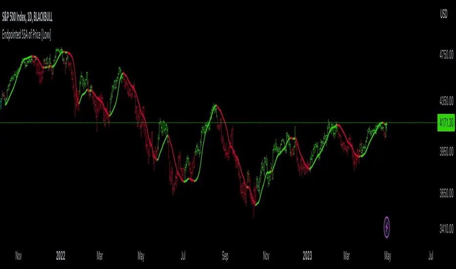
GKD-C EP SSA of Normalized Price [Loxx]The Giga Kaleidoscope GKD-C EP SSA of Normalized Price is a confirmation module included in Loxx's "Giga Kaleidoscope Modularized Trading System."
█ GKD-C End Pointed SSA of Normalized Price
Caterpillar SSA is a variant of Singular Spectrum Analysis (SSA) that is specifically designed for time series with missing values. It is a non-parametric method that decomposes a time series into a set of interpretable components, each having a meaningful interpretation. These components can then be used for a variety of machine learning tasks, such as:
Forecasting: By identifying the trend and seasonality components of a time series, Caterpillar SSA can be used to forecast future values.
Anomaly detection: By identifying unusual spikes or dips in a time series, Caterpillar SSA can be used to detect anomalies.
Feature extraction: The components extracted by Caterpillar SSA can be used as features for other machine learning models, such as neural networks.
In addition to its ability to handle missing values, Caterpillar SSA is also a relatively computationally efficient method. This makes it a good choice for large and complex time series datasets.
Here are some examples of how Caterpillar SSA has been used in machine learning:
In a study of financial markets, Caterpillar SSA was used to forecast stock prices. The results showed that the method was able to improve forecasting accuracy over traditional methods.
2017 paper by Danilov, Zhigljavsky, and Nekrutkin entitled "Caterpillar SSA: A New Tool for Forecasting Financial Time Series." The paper can be found here: arxiv.org
In a study of climate data, Caterpillar SSA was used to detect anomalous weather patterns. The results showed that the method was able to identify patterns that were not visible to the naked eye.
2018 paper by Wang, Zhang, and Wang entitled "Caterpillar SSA for Anomaly Detection in Climate Data." The paper can be found here: arxiv.org
In a study of sensor data, Caterpillar SSA was used to extract features for a machine learning model that was used to classify different types of objects. The results showed that the method was able to extract features that were more informative than those extracted by traditional methods.
2019 paper by Zhang, Zhou, and Zhang entitled "Caterpillar SSA for Feature Extraction in Sensor Data." The paper can be found here: arxiv.org
Caterpillar SSA is a powerful tool that can be used for a variety of machine learning tasks. It is particularly well-suited for time series datasets with missing values.
For our purposes here, SSA is used to create a smoothed oscillator of price. This indicator requires a lot of processing power and as such this indicator is restricted to XX bars back so that it will even load on the screen.
█ Giga Kaleidoscope Modularized Trading System
Core components of an NNFX algorithmic trading strategy
The NNFX algorithm is built on the principles of trend, momentum, and volatility. There are six core components in the NNFX trading algorithm:
1. Volatility - price volatility; e.g., Average True Range, True Range Double, Close-to-Close, etc.
2. Baseline - a moving average to identify price trend
3. Confirmation 1 - a technical indicator used to identify trends
4. Confirmation 2 - a technical indicator used to identify trends
5. Continuation - a technical indicator used to identify trends
6. Volatility/Volume - a technical indicator used to identify volatility/volume breakouts/breakdown
7. Exit - a technical indicator used to determine when a trend is exhausted
8. Metamorphosis - a technical indicator that produces a compound signal from the combination of other GKD indicators*
*(not part of the NNFX algorithm)
What is Volatility in the NNFX trading system?
In the NNFX (No Nonsense Forex) trading system, ATR (Average True Range) is typically used to measure the volatility of an asset. It is used as a part of the system to help determine the appropriate stop loss and take profit levels for a trade. ATR is calculated by taking the average of the true range values over a specified period.
True range is calculated as the maximum of the following values:
-Current high minus the current low
-Absolute value of the current high minus the previous close
-Absolute value of the current low minus the previous close
ATR is a dynamic indicator that changes with changes in volatility. As volatility increases, the value of ATR increases, and as volatility decreases, the value of ATR decreases. By using ATR in NNFX system, traders can adjust their stop loss and take profit levels according to the volatility of the asset being traded. This helps to ensure that the trade is given enough room to move, while also minimizing potential losses.
Other types of volatility include True Range Double (TRD), Close-to-Close, and Garman-Klass
What is a Baseline indicator?
The baseline is essentially a moving average, and is used to determine the overall direction of the market.
The baseline in the NNFX system is used to filter out trades that are not in line with the long-term trend of the market. The baseline is plotted on the chart along with other indicators, such as the Moving Average (MA), the Relative Strength Index (RSI), and the Average True Range (ATR).
Trades are only taken when the price is in the same direction as the baseline. For example, if the baseline is sloping upwards, only long trades are taken, and if the baseline is sloping downwards, only short trades are taken. This approach helps to ensure that trades are in line with the overall trend of the market, and reduces the risk of entering trades that are likely to fail.
By using a baseline in the NNFX system, traders can have a clear reference point for determining the overall trend of the market, and can make more informed trading decisions. The baseline helps to filter out noise and false signals, and ensures that trades are taken in the direction of the long-term trend.
What is a Confirmation indicator?
Confirmation indicators are technical indicators that are used to confirm the signals generated by primary indicators. Primary indicators are the core indicators used in the NNFX system, such as the Average True Range (ATR), the Moving Average (MA), and the Relative Strength Index (RSI).
The purpose of the confirmation indicators is to reduce false signals and improve the accuracy of the trading system. They are designed to confirm the signals generated by the primary indicators by providing additional information about the strength and direction of the trend.
Some examples of confirmation indicators that may be used in the NNFX system include the Bollinger Bands, the MACD (Moving Average Convergence Divergence), and the MACD Oscillator. These indicators can provide information about the volatility, momentum, and trend strength of the market, and can be used to confirm the signals generated by the primary indicators.
In the NNFX system, confirmation indicators are used in combination with primary indicators and other filters to create a trading system that is robust and reliable. By using multiple indicators to confirm trading signals, the system aims to reduce the risk of false signals and improve the overall profitability of the trades.
What is a Continuation indicator?
In the NNFX (No Nonsense Forex) trading system, a continuation indicator is a technical indicator that is used to confirm a current trend and predict that the trend is likely to continue in the same direction. A continuation indicator is typically used in conjunction with other indicators in the system, such as a baseline indicator, to provide a comprehensive trading strategy.
What is a Volatility/Volume indicator?
Volume indicators, such as the On Balance Volume (OBV), the Chaikin Money Flow (CMF), or the Volume Price Trend (VPT), are used to measure the amount of buying and selling activity in a market. They are based on the trading volume of the market, and can provide information about the strength of the trend. In the NNFX system, volume indicators are used to confirm trading signals generated by the Moving Average and the Relative Strength Index. Volatility indicators include Average Direction Index, Waddah Attar, and Volatility Ratio. In the NNFX trading system, volatility is a proxy for volume and vice versa.
By using volume indicators as confirmation tools, the NNFX trading system aims to reduce the risk of false signals and improve the overall profitability of trades. These indicators can provide additional information about the market that is not captured by the primary indicators, and can help traders to make more informed trading decisions. In addition, volume indicators can be used to identify potential changes in market trends and to confirm the strength of price movements.
What is an Exit indicator?
The exit indicator is used in conjunction with other indicators in the system, such as the Moving Average (MA), the Relative Strength Index (RSI), and the Average True Range (ATR), to provide a comprehensive trading strategy.
The exit indicator in the NNFX system can be any technical indicator that is deemed effective at identifying optimal exit points. Examples of exit indicators that are commonly used include the Parabolic SAR, the Average Directional Index (ADX), and the Chandelier Exit.
The purpose of the exit indicator is to identify when a trend is likely to reverse or when the market conditions have changed, signaling the need to exit a trade. By using an exit indicator, traders can manage their risk and prevent significant losses.
In the NNFX system, the exit indicator is used in conjunction with a stop loss and a take profit order to maximize profits and minimize losses. The stop loss order is used to limit the amount of loss that can be incurred if the trade goes against the trader, while the take profit order is used to lock in profits when the trade is moving in the trader's favor.
Overall, the use of an exit indicator in the NNFX trading system is an important component of a comprehensive trading strategy. It allows traders to manage their risk effectively and improve the profitability of their trades by exiting at the right time.
What is an Metamorphosis indicator?
The concept of a metamorphosis indicator involves the integration of two or more GKD indicators to generate a compound signal. This is achieved by evaluating the accuracy of each indicator and selecting the signal from the indicator with the highest accuracy. As an illustration, let's consider a scenario where we calculate the accuracy of 10 indicators and choose the signal from the indicator that demonstrates the highest accuracy.
The resulting output from the metamorphosis indicator can then be utilized in a GKD-BT backtest by occupying a slot that aligns with the purpose of the metamorphosis indicator. The slot can be a GKD-B, GKD-C, or GKD-E slot, depending on the specific requirements and objectives of the indicator. This allows for seamless integration and utilization of the compound signal within the GKD-BT framework.
How does Loxx's GKD (Giga Kaleidoscope Modularized Trading System) implement the NNFX algorithm outlined above?
Loxx's GKD v2.0 system has five types of modules (indicators/strategies). These modules are:
1. GKD-BT - Backtesting module (Volatility, Number 1 in the NNFX algorithm)
2. GKD-B - Baseline module (Baseline and Volatility/Volume, Numbers 1 and 2 in the NNFX algorithm)
3. GKD-C - Confirmation 1/2 and Continuation module (Confirmation 1/2 and Continuation, Numbers 3, 4, and 5 in the NNFX algorithm)
4. GKD-V - Volatility/Volume module (Confirmation 1/2, Number 6 in the NNFX algorithm)
5. GKD-E - Exit module (Exit, Number 7 in the NNFX algorithm)
6. GKD-M - Metamorphosis module (Metamorphosis, Number 8 in the NNFX algorithm, but not part of the NNFX algorithm)
(additional module types will added in future releases)
Each module interacts with every module by passing data to A backtest module wherein the various components of the GKD system are combined to create a trading signal.
That is, the Baseline indicator passes its data to Volatility/Volume. The Volatility/Volume indicator passes its values to the Confirmation 1 indicator. The Confirmation 1 indicator passes its values to the Confirmation 2 indicator. The Confirmation 2 indicator passes its values to the Continuation indicator. The Continuation indicator passes its values to the Exit indicator, and finally, the Exit indicator passes its values to the Backtest strategy.
This chaining of indicators requires that each module conform to Loxx's GKD protocol, therefore allowing for the testing of every possible combination of technical indicators that make up the six components of the NNFX algorithm.
What does the application of the GKD trading system look like?
Example trading system:
Backtest: Multi-Ticker CC Backtest
Baseline: Hull Moving Average
Volatility/Volume: Hurst Exponent
Confirmation 1: EP SSA of Normalized Price as shown on the chart above
Confirmation 2: uf2018
Continuation: Coppock Curve
Exit: Rex Oscillator
Metamorphosis: Baseline Optimizer
Each GKD indicator is denoted with a module identifier of either: GKD-BT, GKD-B, GKD-C, GKD-V, GKD-M, or GKD-E. This allows traders to understand to which module each indicator belongs and where each indicator fits into the GKD system.
█ Giga Kaleidoscope Modularized Trading System Signals
Standard Entry
1. GKD-C Confirmation gives signal
2. Baseline agrees
3. Price inside Goldie Locks Zone Minimum
4. Price inside Goldie Locks Zone Maximum
5. Confirmation 2 agrees
6. Volatility/Volume agrees
1-Candle Standard Entry
1a. GKD-C Confirmation gives signal
2a. Baseline agrees
3a. Price inside Goldie Locks Zone Minimum
4a. Price inside Goldie Locks Zone Maximum
Next Candle
1b. Price retraced
2b. Baseline agrees
3b. Confirmation 1 agrees
4b. Confirmation 2 agrees
5b. Volatility/Volume agrees
Baseline Entry
1. GKD-B Baseline gives signal
2. Confirmation 1 agrees
3. Price inside Goldie Locks Zone Minimum
4. Price inside Goldie Locks Zone Maximum
5. Confirmation 2 agrees
6. Volatility/Volume agrees
7. Confirmation 1 signal was less than 'Maximum Allowable PSBC Bars Back' prior
1-Candle Baseline Entry
1a. GKD-B Baseline gives signal
2a. Confirmation 1 agrees
3a. Price inside Goldie Locks Zone Minimum
4a. Price inside Goldie Locks Zone Maximum
5a. Confirmation 1 signal was less than 'Maximum Allowable PSBC Bars Back' prior
Next Candle
1b. Price retraced
2b. Baseline agrees
3b. Confirmation 1 agrees
4b. Confirmation 2 agrees
5b. Volatility/Volume agrees
Volatility/Volume Entry
1. GKD-V Volatility/Volume gives signal
2. Confirmation 1 agrees
3. Price inside Goldie Locks Zone Minimum
4. Price inside Goldie Locks Zone Maximum
5. Confirmation 2 agrees
6. Baseline agrees
7. Confirmation 1 signal was less than 7 candles prior
1-Candle Volatility/Volume Entry
1a. GKD-V Volatility/Volume gives signal
2a. Confirmation 1 agrees
3a. Price inside Goldie Locks Zone Minimum
4a. Price inside Goldie Locks Zone Maximum
5a. Confirmation 1 signal was less than 'Maximum Allowable PSVVC Bars Back' prior
Next Candle
1b. Price retraced
2b. Volatility/Volume agrees
3b. Confirmation 1 agrees
4b. Confirmation 2 agrees
5b. Baseline agrees
Confirmation 2 Entry
1. GKD-C Confirmation 2 gives signal
2. Confirmation 1 agrees
3. Price inside Goldie Locks Zone Minimum
4. Price inside Goldie Locks Zone Maximum
5. Volatility/Volume agrees
6. Baseline agrees
7. Confirmation 1 signal was less than 7 candles prior
1-Candle Confirmation 2 Entry
1a. GKD-C Confirmation 2 gives signal
2a. Confirmation 1 agrees
3a. Price inside Goldie Locks Zone Minimum
4a. Price inside Goldie Locks Zone Maximum
5a. Confirmation 1 signal was less than 'Maximum Allowable PSC2C Bars Back' prior
Next Candle
1b. Price retraced
2b. Confirmation 2 agrees
3b. Confirmation 1 agrees
4b. Volatility/Volume agrees
5b. Baseline agrees
PullBack Entry
1a. GKD-B Baseline gives signal
2a. Confirmation 1 agrees
3a. Price is beyond 1.0x Volatility of Baseline
Next Candle
1b. Price inside Goldie Locks Zone Minimum
2b. Price inside Goldie Locks Zone Maximum
3b. Confirmation 1 agrees
4b. Confirmation 2 agrees
5b. Volatility/Volume agrees
Continuation Entry
1. Standard Entry, 1-Candle Standard Entry, Baseline Entry, 1-Candle Baseline Entry, Volatility/Volume Entry, 1-Candle Volatility/Volume Entry, Confirmation 2 Entry, 1-Candle Confirmation 2 Entry, or Pullback entry triggered previously
2. Baseline hasn't crossed since entry signal trigger
4. Confirmation 1 agrees
5. Baseline agrees
6. Confirmation 2 agrees

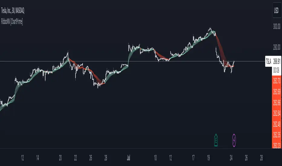
RibboNN Machine Learning [ChartPrime]The RibboNN ML indicator is a powerful tool designed to predict the direction of the market and display it through a ribbon-like visual representation, with colors changing based on the prediction outcome from a conditional class. The primary focus of this indicator is to assist traders in trend following trading strategies.
The RibboNN ML in action
Prediction Process:
Conditional Class: The indicator's predictive model relies on a conditional class, which combines information from both longcon (long condition) and short condition. These conditions are determined using specific rules and criteria, taking into account various market factors and indicators.
Direction Prediction: The conditional class provides the basis for predicting the direction of the market move. When the prediction value is greater than 0, it indicates an upward trend, while a value less than 0 suggests a downward trend.
Nearest Neighbor (NN): To attempt to enhance the accuracy of predictions, the RibboNN ML indicator incorporates a Nearest Neighbor algorithm. This algorithm analyzes historical data from the Ribbon ML's predictive model (RMF) and identifies patterns that closely resemble the current conditional prediction class, thereby offering more robust trend forecasts.
Ribbon Visualization:
The Ribbon ML indicator visually represents its predictions through a ribbon-like display. The ribbon changes colors based on the direction predicted by the conditional class. An upward trend is represented by a green color, while a downward trend is depicted by a red color, allowing traders to quickly identify potential market directions.
The introduction of the Nearest Neighbor algorithm provides the Ribbon ML indicator with unique and adaptive behaviors. By dynamically analyzing historical patterns and incorporating them into predictions, the indicator can adapt to changing market conditions and offer more reliable signals for trend following trading strategies.
Manipulation of the NN Settings:
Smaller Value of Neighbours Count:
When the value of "Neighbours Count" is small, the algorithm considers only a few nearest neighbors for making predictions.
A smaller value of "Neighbours Count" leads to more flexible decision boundaries, which can result in a more granular and sensitive model.
However, using a very small value might lead to overfitting, especially if the training data contains noise or outliers.
Larger Value of "Neighbours Count":
When the value of "Neighbours Count" is large, the algorithm considers a larger number of nearest neighbors for making predictions.
A larger value of "Neighbours Count" leads to smoother decision boundaries and helps capture the global patterns in the data.
However, setting a very large value might result in a loss of local patterns and make the model less sensitive to changes in the data.
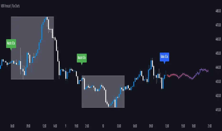
Wick-to-Body Ratio Trend Forecast | Flux ChartsThe Wick-to-Body Ratio Trend Forecast Indicator aims to forecast potential movements following the last closed candle using the wick-to-body ratio. The script identifies those candles within the loopback period with a ratio matching that of the last closed candle and provides an analysis of their trends.
➡️ USAGE
Wick-to-body ratios can be used in many strategies. The most common use in stock trading is to discern bullish or bearish sentiment. This indicator extends candle ratios, revealing previous patterns that follow a candle with a similar ratio. The most basic use of this indicator is the single forecast line.
➡️ FORECASTING SYSTEM
This line displays a compilation of the averages of all the previous trends resulting from those historical candles with a matching ratio. It shows the average movements of the trends as well as the 'strength' of the trend. The 'strength' of the trend is a gradient that is blue when the trend deviates more from the average and red when it deviates less.
Chart: AMEX:SPY 30 min; Indicator Settings: Loopback 700, Previous Trends ON
The color-coded deviation is visible in this image of the indicator with the default settings (except for Forecast Lines > Previous Trends ), and the trend line grows bluer as the past patterns deviate more.
➡️ ADAPTIVE ACCEPTABLE RANGE
The algorithm looks back at every candle within the loopback period to find candles that match the last closed candle. The algorithm adaptively changes the acceptable range to which a candle can differ from the ratio of the last closed candle. The algorithm will never have more than 15 historical points used, as it will lower its sensitivity before it reaches that point.
Chart: BITSTAMP:BTCUSD 5 min; Indicator Settings: Loopback 700
Here is the BTC chart on 7/6/23 with default settings except for the loopback period at 700.
Chart: BITSTAMP:BTCUSD 5 min; Indicator Settings: Loopback 200
Here is the exact same chart with a loopback period of 200. While the first ratio for both is the same, a new ratio is revealed for the chart with a loopback of only 200 because the adaptive range is adjusted in the algorithm to find an acceptable number of reference points. Note the table in the top right however, while the algorithm adapts the acceptable range between the current ratio and historical ones to find reference points, there is a threshold at which candles will be considered too inaccurate to be considered. This prevents meaningless associations between candles due to a particularly rare ratio. This threshold can be adjusted in the settings through "Default Accuracy".
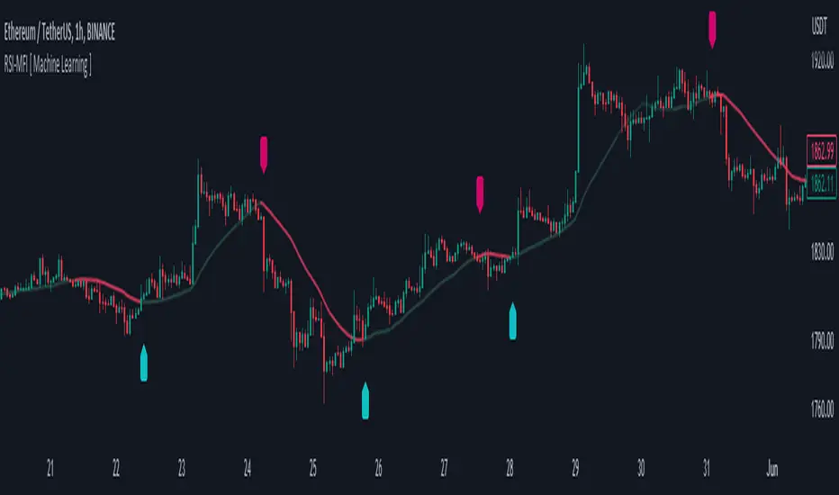
RSI-MFI Machine Learning [ Manhattan distance ]The RSI-MFI Machine Learning Indicator is a technical analysis tool that combines the Relative Strength Index (RSI) and Money Flow Index (MFI) indicators with the Manhattan distance metric.
It aims to provide insights into potential trade setups by leveraging machine learning principles and calculating distances between current and historical data points.
The indicator starts by calculating the RSI and MFI values based on the specified periods for each indicator.
The RSI measures the strength and speed of price movements, while the MFI evaluates the inflow and outflow of money in the market.
By combining these two indicators, the indicator captures both price momentum and money flow dynamics.
To apply machine learning principles , the indicator utilizes the Manhattan distance metric to quantify the similarity or dissimilarity between different data points.
The Manhattan distance is calculated by taking the absolute differences between corresponding RSI and MFI values of the current point and historical points.
Next, the indicator determines the nearest neighbors based on the calculated Manhattan distances.
The number of nearest neighbors is determined by the square root of the specified count of neighbors.
By identifying similar patterns and behaviors in the historical data, the indicator aims to uncover potential trade opportunities.
Trade signals are generated based on the calculated distances. The indicator compares each distance with the maximum distance encountered so far.
If a new maximum distance is found, it updates the value and considers the corresponding direction as a potential trade signal. The trade signals are stored in an array for further analysis.
Furthermore, the indicator considers the price action and a calculated regression line to differentiate between long and short trade signals.
Long trade signals are identified when the closing price is above the regression line, indicating a potentially bullish setup.
Short trade signals are identified when the closing price is below the regression line, indicating a potentially bearish setup.
The RSI-MFI Machine Learning Indicator visualizes the regression line on the price chart and labels the bars accordingly. It highlights the regression line with different colors based on the trade signals, making it easier for traders to identify potential entry or exit points.
Traders can use the RSI-MFI Machine Learning Indicator as a tool to analyze price movements, evaluate market conditions based on RSI and MFI, leverage machine learning concepts to find similar patterns, and make informed trading decisions.
Machine Learning : Torben's Moving Median KNN BandsWhat is Median Filtering ?
Median filtering is a non-linear digital filtering technique, often used to remove noise from an image or signal. Such noise reduction is a typical pre-processing step to improve the results of later processing (for example, edge detection on an image). Median filtering is very widely used in digital image processing because, under certain conditions, it preserves edges while removing noise (but see the discussion below), also having applications in signal processing.
The main idea of the median filter is to run through the signal entry by entry, replacing each entry with the median of neighboring entries. The pattern of neighbors is called the "window", which slides, entry by entry, over the entire signal. For one-dimensional signals, the most obvious window is just the first few preceding and following entries, whereas for two-dimensional (or higher-dimensional) data the window must include all entries within a given radius or ellipsoidal region (i.e. the median filter is not a separable filter).
The median filter works by taking the median of all the pixels in a neighborhood around the current pixel. The median is the middle value in a sorted list of numbers. This means that the median filter is not sensitive to the order of the pixels in the neighborhood, and it is not affected by outliers (very high or very low values).
The median filter is a very effective way to remove noise from images. It can remove both salt and pepper noise (random white and black pixels) and Gaussian noise (randomly distributed pixels with a Gaussian distribution). The median filter is also very good at preserving edges, which is why it is often used as a pre-processing step for edge detection.
However, the median filter can also blur images. This is because the median filter replaces each pixel with the value of the median of its neighbors. This can cause the edges of objects in the image to be smoothed out. The amount of blurring depends on the size of the window used by the median filter. A larger window will blur more than a smaller window.
The median filter is a very versatile tool that can be used for a variety of tasks in image processing. It is a good choice for removing noise and preserving edges, but it can also blur images. The best way to use the median filter is to experiment with different window sizes to find the setting that produces the desired results.
What is this Indicator ?
K-nearest neighbors (KNN) is a simple, non-parametric machine learning algorithm that can be used for both classification and regression tasks. The basic idea behind KNN is to find the K most similar data points to a new data point and then use the labels of those K data points to predict the label of the new data point.
Torben's moving median is a variation of the median filter that is used to remove noise from images. The median filter works by replacing each pixel in an image with the median of its neighbors. Torben's moving median works in a similar way, but it also averages the values of the neighbors. This helps to reduce the amount of blurring that can occur with the median filter.
KNN over Torben's moving median is a hybrid algorithm that combines the strengths of both KNN and Torben's moving median. KNN is able to learn the underlying distribution of the data, while Torben's moving median is able to remove noise from the data. This combination can lead to better performance than either algorithm on its own.
To implement KNN over Torben's moving median, we first need to choose a value for K. The value of K controls how many neighbors are used to predict the label of a new data point. A larger value of K will make the algorithm more robust to noise, but it will also make the algorithm less sensitive to local variations in the data.
Once we have chosen a value for K, we need to train the algorithm on a dataset of labeled data points. The training dataset will be used to learn the underlying distribution of the data.
Once the algorithm is trained, we can use it to predict the labels of new data points. To do this, we first need to find the K most similar data points to the new data point. We can then use the labels of those K data points to predict the label of the new data point.
KNN over Torben's moving median is a simple, yet powerful algorithm that can be used for a variety of tasks. It is particularly well-suited for tasks where the data is noisy or where the underlying distribution of the data is unknown.
Here are some of the advantages of using KNN over Torben's moving median:
KNN is able to learn the underlying distribution of the data.
KNN is robust to noise.
KNN is not sensitive to local variations in the data.
Here are some of the disadvantages of using KNN over Torben's moving median:
KNN can be computationally expensive for large datasets.
KNN can be sensitive to the choice of K.
KNN can be slow to train.

Machine Learning : Dominant Cycle Elastic Volume KNNAbout the Script
Dominant Cycle Elastic Volume KNN ,
is a non-parametric algorithm, which means that, initially it makes no assumptions about the underlying distribution of the time-series price as well as volume.
This approach gives it flexibility so that it can be used on a wide variety of securities at variety of timeframes.(even on lower timeframes such as seconds)
The main purpose of this indicator is to predict the trend of the underlying, by converging price, volume and dominant cycle as dimensions and generate signals of action.
Key terms :
Dominant cycle is a time cycle that has a greater influence on the overall behaviour of a system than other cycles.
The system uses Ehlers method to calculate Dominant Cycle/ Period.
Dominant cycle is used to determine the influencing period for the underlying.
Once the dominant cycle/ period is identified, it is treated as a dynamic length for considering further calculations
Elastic Volume MA is a volume based moving average which is generally used to converge the volume with price, the dominant period is used here as the length parameter
KNN K-Nearest Neighbour is one of the simplest Machine Learning algorithms based on Supervised Learning technique.
K-NN algorithm assumes the similarity between the new case/data and available cases and put the new case into the category that is most similar to the available categories.
K-NN algorithm stores all the available data and classifies a new data point based on the similarity. This means when new data appears then it can be easily classified into a well suite category by using K- NN algorithm. K-NN algorithm can be used for Regression as well as for Classification but mostly it is used for the Classification problems.
So, K-NN is used here to classify the trend of the Dominant Cycle Elastic Volume, and Generate Signals on top of it
How to Use the Indicator ?
The Buy Signal Candle
The Sell Signal Candle
The Buy Setup
The Sell Setup
Stop and Reverse Structure
What Timeframes and Symbols can this indicator be used on ?
The above indicator can be used on any liquid security which has volume information intact with ticker
and it can be used on any timeframe, but the best timeframes are
The indicator can also be used as a trend confirmatory indicators on lower time frames, like 30second
The Script has provision for alerts
Two alerts are there :
Alert 1= "LONG CONDITION : DCEV-ML"
Alert 2= "SHORT CONDITION : DCEV-ML"
How to request for access ?
Simply private message me !

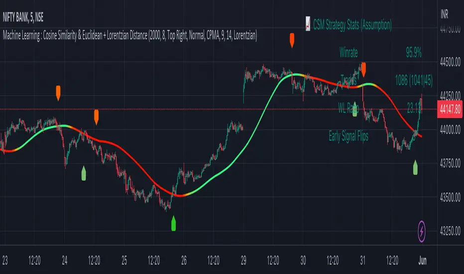
Machine Learning : Cosine Similarity & Euclidean DistanceIntroduction:
This script implements a comprehensive trading strategy that adheres to the established rules and guidelines of housing trading. It leverages advanced machine learning techniques and incorporates customised moving averages, including the Conceptive Price Moving Average (CPMA), to provide accurate signals for informed trading decisions in the housing market. Additionally, signal processing techniques such as Lorentzian, Euclidean distance, Cosine similarity, Know sure thing, Rational Quadratic, and sigmoid transformation are utilised to enhance the signal quality and improve trading accuracy.
Features:
Market Analysis: The script utilizes advanced machine learning methods such as Lorentzian, Euclidean distance, and Cosine similarity to analyse market conditions. These techniques measure the similarity and distance between data points, enabling more precise signal identification and enhancing trading decisions.
Cosine similarity:
Cosine similarity is a measure used to determine the similarity between two vectors, typically in a high-dimensional space. It calculates the cosine of the angle between the vectors, indicating the degree of similarity or dissimilarity.
In the context of trading or signal processing, cosine similarity can be employed to compare the similarity between different data points or signals. The vectors in this case represent the numerical representations of the data points or signals.
Cosine similarity ranges from -1 to 1, with 1 indicating perfect similarity, 0 indicating no similarity, and -1 indicating perfect dissimilarity. A higher cosine similarity value suggests a closer match between the vectors, implying that the signals or data points share similar characteristics.
Lorentzian Classification:
Lorentzian classification is a machine learning algorithm used for classification tasks. It is based on the Lorentzian distance metric, which measures the similarity or dissimilarity between two data points. The Lorentzian distance takes into account the shape of the data distribution and can handle outliers better than other distance metrics.
Euclidean Distance:
Euclidean distance is a distance metric widely used in mathematics and machine learning. It calculates the straight-line distance between two points in Euclidean space. In two-dimensional space, the Euclidean distance between two points (x1, y1) and (x2, y2) is calculated using the formula sqrt((x2 - x1)^2 + (y2 - y1)^2).
Dynamic Time Windows: The script incorporates a dynamic time window function that allows users to define specific time ranges for trading. It checks if the current time falls within the specified window to execute the relevant trading signals.
Custom Moving Averages: The script includes the CPMA, a powerful moving average calculation. Unlike traditional moving averages, the CPMA provides improved support and resistance levels by considering multiple price types and employing a combination of Exponential Moving Averages (EMAs) and Simple Moving Averages (SMAs). Its adaptive nature ensures responsiveness to changes in price trends.
Signal Processing Techniques: The script applies signal processing techniques such as Know sure thing, Rational Quadratic, and sigmoid transformation to enhance the quality of the generated signals. These techniques improve the accuracy and reliability of the trading signals, aiding in making well-informed trading decisions.
Trade Statistics and Metrics: The script provides comprehensive trade statistics and metrics, including total wins, losses, win rate, win-loss ratio, and early signal flips. These metrics offer valuable insights into the performance and effectiveness of the trading strategy.
Usage:
Configuring Time Windows: Users can customize the time windows by specifying the start and finish time ranges according to their trading preferences and local market conditions.
Signal Interpretation: The script generates long and short signals based on the analysis, custom moving averages, and signal processing techniques. Users should pay attention to these signals and take appropriate action, such as entering or exiting trades, depending on their trading strategies.
Trade Statistics: The script continuously tracks and updates trade statistics, providing users with a clear overview of their trading performance. These statistics help users assess the effectiveness of the strategy and make informed decisions.
Conclusion:
With its adherence to housing trading rules, advanced machine learning methods, customized moving averages like the CPMA, and signal processing techniques such as Lorentzian, Euclidean distance, Cosine similarity, Know sure thing, Rational Quadratic, and sigmoid transformation, this script offers users a powerful tool for housing market analysis and trading. By leveraging the provided signals, time windows, and trade statistics, users can enhance their trading strategies and improve their overall trading performance.
Disclaimer:
Please note that while this script incorporates established tradingview housing rules, advanced machine learning techniques, customized moving averages, and signal processing techniques, it should be used for informational purposes only. Users are advised to conduct their own analysis and exercise caution when making trading decisions. The script's performance may vary based on market conditions, user settings, and the accuracy of the machine learning methods and signal processing techniques. The trading platform and developers are not responsible for any financial losses incurred while using this script.
By publishing this script on the platform, traders can benefit from its professional presentation, clear instructions, and the utilisation of advanced machine learning techniques, customised moving averages, and signal processing techniques for enhanced trading signals and accuracy.
I extend my gratitude to TradingView, LUX ALGO, and JDEHORTY for their invaluable contributions to the trading community. Their innovative scripts, meticulous coding patterns, and insightful ideas have profoundly enriched traders' strategies, including my own.
N-Rho To Noise (Reinforcement Learning)N-Rho To Noise is a ratio of 2 components. Rho is my own calculation of a signal that is differenced (force time series stationary, allowing for more predictability) and its relation to a unit of a measure of noise. N is the amount of times it is differenced. Using a simplified q-learning reinforcement learning agent, the length of the ratio is calibrated to its optimal value.
- Purple indicates the undifferenced signal is above the RMSE error bands
- Red indicates both the differenced and undifferenced signals are above the threshold for a strong positive deviation, suggesting a short
- Blue indicates the undifferenced signal is below the RMSE error bands
- Green indicates both the differenced and undifferenced signals are below the threshold for a negative strong deviation, suggesting a long
- Strong long signal when you have both an undifferenced Rho and differenced Rho giving you local agreement (blue bar followed by green)
- Strong short signal when you have an undifferenced and differenced Rho giving you identical signals (purple bar followed by red)
Optimal length: the parameter of the length that the model configures to be the best parameter
Optimal reward: the reward corresponding to the optimal length (green=strong value, orange=intermediate strength, red=poor)
Average reward: the average reward of the set of lengths used over all episodes (green=strong value, orange=intermediate strength, red=poor)
Cumulative reward: the sum of all the rewards
Variance: a measure of how varied the data is (too much variance can suggest it cannot generalize too well to unseen data)

Endpointed SSA of Price [Loxx]The Endpointed SSA of Price: A Comprehensive Tool for Market Analysis and Decision-Making
The financial markets present sophisticated challenges for traders and investors as they navigate the complexities of market behavior. To effectively interpret and capitalize on these complexities, it is crucial to employ powerful analytical tools that can reveal hidden patterns and trends. One such tool is the Endpointed SSA of Price, which combines the strengths of Caterpillar Singular Spectrum Analysis, a sophisticated time series decomposition method, with insights from the fields of economics, artificial intelligence, and machine learning.
The Endpointed SSA of Price has its roots in the interdisciplinary fusion of mathematical techniques, economic understanding, and advancements in artificial intelligence. This unique combination allows for a versatile and reliable tool that can aid traders and investors in making informed decisions based on comprehensive market analysis.
The Endpointed SSA of Price is not only valuable for experienced traders but also serves as a useful resource for those new to the financial markets. By providing a deeper understanding of market forces, this innovative indicator equips users with the knowledge and confidence to better assess risks and opportunities in their financial pursuits.
█ Exploring Caterpillar SSA: Applications in AI, Machine Learning, and Finance
Caterpillar SSA (Singular Spectrum Analysis) is a non-parametric method for time series analysis and signal processing. It is based on a combination of principles from classical time series analysis, multivariate statistics, and the theory of random processes. The method was initially developed in the early 1990s by a group of Russian mathematicians, including Golyandina, Nekrutkin, and Zhigljavsky.
Background Information:
SSA is an advanced technique for decomposing time series data into a sum of interpretable components, such as trend, seasonality, and noise. This decomposition allows for a better understanding of the underlying structure of the data and facilitates forecasting, smoothing, and anomaly detection. Caterpillar SSA is a particular implementation of SSA that has proven to be computationally efficient and effective for handling large datasets.
Uses in AI and Machine Learning:
In recent years, Caterpillar SSA has found applications in various fields of artificial intelligence (AI) and machine learning. Some of these applications include:
1. Feature extraction: Caterpillar SSA can be used to extract meaningful features from time series data, which can then serve as inputs for machine learning models. These features can help improve the performance of various models, such as regression, classification, and clustering algorithms.
2. Dimensionality reduction: Caterpillar SSA can be employed as a dimensionality reduction technique, similar to Principal Component Analysis (PCA). It helps identify the most significant components of a high-dimensional dataset, reducing the computational complexity and mitigating the "curse of dimensionality" in machine learning tasks.
3. Anomaly detection: The decomposition of a time series into interpretable components through Caterpillar SSA can help in identifying unusual patterns or outliers in the data. Machine learning models trained on these decomposed components can detect anomalies more effectively, as the noise component is separated from the signal.
4. Forecasting: Caterpillar SSA has been used in combination with machine learning techniques, such as neural networks, to improve forecasting accuracy. By decomposing a time series into its underlying components, machine learning models can better capture the trends and seasonality in the data, resulting in more accurate predictions.
Application in Financial Markets and Economics:
Caterpillar SSA has been employed in various domains within financial markets and economics. Some notable applications include:
1. Stock price analysis: Caterpillar SSA can be used to analyze and forecast stock prices by decomposing them into trend, seasonal, and noise components. This decomposition can help traders and investors better understand market dynamics, detect potential turning points, and make more informed decisions.
2. Economic indicators: Caterpillar SSA has been used to analyze and forecast economic indicators, such as GDP, inflation, and unemployment rates. By decomposing these time series, researchers can better understand the underlying factors driving economic fluctuations and develop more accurate forecasting models.
3. Portfolio optimization: By applying Caterpillar SSA to financial time series data, portfolio managers can better understand the relationships between different assets and make more informed decisions regarding asset allocation and risk management.
Application in the Indicator:
In the given indicator, Caterpillar SSA is applied to a financial time series (price data) to smooth the series and detect significant trends or turning points. The method is used to decompose the price data into a set number of components, which are then combined to generate a smoothed signal. This signal can help traders and investors identify potential entry and exit points for their trades.
The indicator applies the Caterpillar SSA method by first constructing the trajectory matrix using the price data, then computing the singular value decomposition (SVD) of the matrix, and finally reconstructing the time series using a selected number of components. The reconstructed series serves as a smoothed version of the original price data, highlighting significant trends and turning points. The indicator can be customized by adjusting the lag, number of computations, and number of components used in the reconstruction process. By fine-tuning these parameters, traders and investors can optimize the indicator to better match their specific trading style and risk tolerance.
Caterpillar SSA is versatile and can be applied to various types of financial instruments, such as stocks, bonds, commodities, and currencies. It can also be combined with other technical analysis tools or indicators to create a comprehensive trading system. For example, a trader might use Caterpillar SSA to identify the primary trend in a market and then employ additional indicators, such as moving averages or RSI, to confirm the trend and generate trading signals.
In summary, Caterpillar SSA is a powerful time series analysis technique that has found applications in AI and machine learning, as well as financial markets and economics. By decomposing a time series into interpretable components, Caterpillar SSA enables better understanding of the underlying structure of the data, facilitating forecasting, smoothing, and anomaly detection. In the context of financial trading, the technique is used to analyze price data, detect significant trends or turning points, and inform trading decisions.
█ Input Parameters
This indicator takes several inputs that affect its signal output. These inputs can be classified into three categories: Basic Settings, UI Options, and Computation Parameters.
Source: This input represents the source of price data, which is typically the closing price of an asset. The user can select other price data, such as opening price, high price, or low price. The selected price data is then utilized in the Caterpillar SSA calculation process.
Lag: The lag input determines the window size used for the time series decomposition. A higher lag value implies that the SSA algorithm will consider a longer range of historical data when extracting the underlying trend and components. This parameter is crucial, as it directly impacts the resulting smoothed series and the quality of extracted components.
Number of Computations: This input, denoted as 'ncomp,' specifies the number of eigencomponents to be considered in the reconstruction of the time series. A smaller value results in a smoother output signal, while a higher value retains more details in the series, potentially capturing short-term fluctuations.
SSA Period Normalization: This input is used to normalize the SSA period, which adjusts the significance of each eigencomponent to the overall signal. It helps in making the algorithm adaptive to different timeframes and market conditions.
Number of Bars: This input specifies the number of bars to be processed by the algorithm. It controls the range of data used for calculations and directly affects the computation time and the output signal.
Number of Bars to Render: This input sets the number of bars to be plotted on the chart. A higher value slows down the computation but provides a more comprehensive view of the indicator's performance over a longer period. This value controls how far back the indicator is rendered.
Color bars: This boolean input determines whether the bars should be colored according to the signal's direction. If set to true, the bars are colored using the defined colors, which visually indicate the trend direction.
Show signals: This boolean input controls the display of buy and sell signals on the chart. If set to true, the indicator plots shapes (triangles) to represent long and short trade signals.
Static Computation Parameters:
The indicator also includes several internal parameters that affect the Caterpillar SSA algorithm, such as Maxncomp, MaxLag, and MaxArrayLength. These parameters set the maximum allowed values for the number of computations, the lag, and the array length, ensuring that the calculations remain within reasonable limits and do not consume excessive computational resources.
█ A Note on Endpionted, Non-repainting Indicators
An endpointed indicator is one that does not recalculate or repaint its past values based on new incoming data. In other words, the indicator's previous signals remain the same even as new price data is added. This is an important feature because it ensures that the signals generated by the indicator are reliable and accurate, even after the fact.
When an indicator is non-repainting or endpointed, it means that the trader can have confidence in the signals being generated, knowing that they will not change as new data comes in. This allows traders to make informed decisions based on historical signals, without the fear of the signals being invalidated in the future.
In the case of the Endpointed SSA of Price, this non-repainting property is particularly valuable because it allows traders to identify trend changes and reversals with a high degree of accuracy, which can be used to inform trading decisions. This can be especially important in volatile markets where quick decisions need to be made.
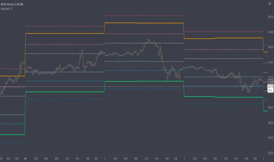
Gamma Bands v. 7.0Gamma Bands are based on previous day data of base intrument, Volatility , Options flow (imported from external source Quandl via TradingView API as TV is not supporting Options as instruments) and few other additional factors to calculate intraday levels. Those levels in correlation with even pure Price Action works like a charm what is confirmed by big orders often placed exactly on those levels on Futures Contracts. We have levels +/- 0.25, 0.5 and 1.0 that are calculated from Pivot Point and are working like Support and Resistance. Higher the number of Gamma, stronger the level. Passing Gamma +1/-1 would be good entry point for trades as almost everytime it is equal to Trend Day. Levels are calculated by Machine Learning algorithm written in Python which downloads data from Options and Darkpool markets, process and calculate levels, export to Quandl and then in PineScript I import the data to indicator. Levels are refreshed each day and are valid for particular trading day.
There's possibility also to enable display of Initial Balance range (High and Low range of bars/candles from 1st hour of regular cash session). Breaking one of extremes of Initial Balance is very often driving sentiment for rest of the session.
Volatility Reversal Levels
They're calculated taking into account Options flow imported to TV (Strikes, Call/Put types & Expiration dates) in combination with Volatility, Volume flow. Based on that we calculate on daily basis Significant Close level and "Stop and Reversal level".
Very often reaching area close to those levels either trigger immediate reversal of previous trend or at least push price into consolidation range.
Lorentzian Classification Strategy Based in the model of Machine learning: Lorentzian Classification by @jdehorty, you will be able to get into trending moves and get interesting entries in the market with this strategy. I also put some new features for better backtesting results!
Backtesting context: 2022-07-19 to 2023-04-14 of US500 1H by PEPPERSTONE. Commissions: 0.03% for each entry, 0.03% for each exit. Risk per trade: 2.5% of the total account
For this strategy, 3 indicators are used:
Machine learning: Lorentzian Classification by @jdehorty
One Ema of 200 periods for identifying the trend
Supertrend indicator as a filter for some exits
Atr stop loss from Gatherio
Trade conditions:
For longs:
Close price is above 200 Ema
Lorentzian Classification indicates a buying signal
This gives us our long signal. Stop loss will be determined by atr stop loss (white point), break even(blue point) by a risk/reward ratio of 1:1 and take profit of 3:1 where half position will be closed. This will be showed as buy.
The other half will be closed when the model indicates a selling signal or Supertrend indicator gives a bearish signal. This will be showed as cl buy.
For shorts:
Close price is under 200 Ema
Lorentzian Classification indicates a selling signal
This gives us our short signal. Stop loss will be determined by atr stop loss (white point), break even(blue point) by a risk/reward ratio of 1:1 and take profit of 3:1 where half position will be closed. This will be showed as sell.
The other half will be closed when the model indicates a buying signal or Supertrend indicator gives a bullish signal. This will be showed as cl sell.
Risk management
To calculate the amount of the position you will use just a small percent of your initial capital for the strategy and you will use the atr stop loss or last swing for this.
Example: You have 1000 usd and you just want to risk 2,5% of your account, there is a buy signal at price of 4,000 usd. The stop loss price from atr stop loss or last swing is 3,900. You calculate the distance in percent between 4,000 and 3,900. In this case, that distance would be of 2.50%. Then, you calculate your position by this way: (initial or current capital * risk per trade of your account) / (stop loss distance).
Using these values on the formula: (1000*2,5%)/(2,5%) = 1000usd. It means, you have to use 1000 usd for risking 2.5% of your account.
We will use this risk management for applying compound interest.
> In settings, with position amount calculator, you can enter the amount in usd of your account and the amount in percentage for risking per trade of the account. You will see this value in green color in the upper left corner that shows the amount in usd to use for risking the specific percentage of your account.
> You can also choose a fixed amount, so you will have to activate fixed amount in risk management for trades and set the fixed amount for backtesting.
Script functions
Inside of settings, you will find some utilities for display atr stop loss, break evens, positions, signals, indicators, a table of some stats from backtesting, etc.
You will find the settings for risk management at the end of the script if you want to change something or trying new values for other assets for backtesting.
If you want to change the initial capital for backtest the strategy, go to properties, and also enter the commisions of your exchange and slippage for more realistic results.
In risk managment you can find an option called "Use leverage ?", activate this if you want to backtest using leverage, which means that in case of not having enough money for risking the % determined by you of your account using your initial capital, you will use leverage for using the enough amount for risking that % of your acount in a buy position. Otherwise, the amount will be limited by your initial/current capital
I also added a function for backtesting if you had added or withdrawn money frequently:
Adding money: You can choose how often you want to add money (Monthly, yearly, daily or weekly). Then a fixed amount of money and activate or deactivate this function
Withdraw money: You can choose if you want to withdraw a fixed amount or a percentage of earnings. Then you can choose a fixed amount of money, the period of time and activate or deactivate this function. Also, the percentage of earnings if you choosed this option.
Some other assets where strategy has worked
BTCUSD 4H, 1D
ETHUSD 4H, 1D
BNBUSD 4H
SPX 1D
BANKNIFTY 4H, 15 min
Some things to consider
USE UNDER YOUR OWN RISK. PAST RESULTS DO NOT REPRESENT THE FUTURE.
DEPENDING OF % ACCOUNT RISK PER TRADE, YOU COULD REQUIRE LEVERAGE FOR OPEN SOME POSITIONS, SO PLEASE, BE CAREFULL AND USE CORRECTLY THE RISK MANAGEMENT
Do not forget to change commissions and other parameters related with back testing results!. If you have problems loading the script reduce max bars back number in general settings
Strategies for trending markets use to have more looses than wins and it takes a long time to get profits, so do not forget to be patient and consistent !
Please, visit the post from @jdehorty called Machine Learning: Lorentzian Classification for a better understanding of his script!
Any support and boosts will be well received. If you have any question, do not doubt to ask!

Lorentzian ML [Sublime Traders]Lorentzian ML
Context: The whole idea of this indicator is to use the Lorentzian Classifier (a popular machine learning model suited for analyzing data in a time series) , add some oscillators and filter them with volume averages in order to get precise swing move indications.
The Lorentzian ML indicator uses the Lorenzian Classifier (LDC) algorithm that takes into account the Commodity Channel Index (CCI) and Relative Strength Index (RSI) signals as raw material to provide buy and sell signals. The indicator is accompanied by take profit , stop loss and entry lines based on the Average True Range (ATR).
Features:
1. Lorentzian Classifier:
Uses the difference between the current and previous values of CCI and RSI to generate buy and sell signals.
The classifier threshold can be adjusted using the input parameter.
2. ATR-based Take Profit Line:
A horizontal take profit line is plotted when buy or sell signals occur.
The line is based on the ATR value and a user-defined multiplier.
3. VMA filtering
Using the simple switches: Scalper, Swing or Holder , the users can easily filter the frequency of the signals in addition to the lookback and threshold filters. This will affect the used VMA lines that use data gathered from multiple timeframes.
Visual Representation:
The indicator plots green candles for buy signals and red candles for sell signals.
Buy and sell labels are displayed on the chart to mark the points where signals occur.
The ATR-based take profit line is displayed in a user-defined color and line width.
Visual representation of the VMA lines : Red - bearish , Blue - uncertain , Green - bullish
Changes and features to come
Fix "holder" switch on sell side that sometimes bugs the whole chart.
Add more intuitive filtering methods.
Add two more oscillators to the Lorentzian pool.
Create switches for Lorentzian source.
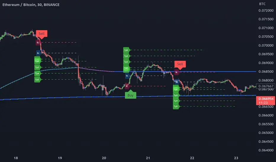
GKD-C Smooth Step [Loxx]Giga Kaleidoscope Smooth Step is a Confirmation module included in Loxx's "Giga Kaleidoscope Modularized Trading System".
█ Giga Kaleidoscope Modularized Trading System
What is Loxx's "Giga Kaleidoscope Modularized Trading System"?
The Giga Kaleidoscope Modularized Trading System is a trading system built on the philosophy of the NNFX (No Nonsense Forex) algorithmic trading.
What is an NNFX algorithmic trading strategy?
The NNFX algorithm is built on the principles of trend, momentum, and volatility. There are six core components in the NNFX trading algorithm:
1. Volatility - price volatility; e.g., Average True Range, True Range Double, Close-to-Close, etc.
2. Baseline - a moving average to identify price trend
3. Confirmation 1 - a technical indicator used to identify trends.
4. Confirmation 2 - a technical indicator used to identify trends.
5. Continuation - a technical indicator used to identify trends.
6. Volatility/Volume - a technical indicator used to identify volatility/volume breakouts/breakdown.
7. Exit - a technical indicator used to determine when a trend is exhausted.
How does Loxx's GKD (Giga Kaleidoscope Modularized Trading System) implement the NNFX algorithm outlined above?
Loxx's GKD v1.0 system has five types of modules (indicators/strategies). These modules are:
1. GKD-BT - Backtesting module (Volatility, Number 1 in the NNFX algorithm)
2. GKD-B - Baseline module (Baseline and Volatility/Volume, Numbers 1 and 2 in the NNFX algorithm)
3. GKD-C - Confirmation 1/2 and Continuation module (Confirmation 1/2 and Continuation, Numbers 3, 4, and 5 in the NNFX algorithm)
4. GKD-V - Volatility/Volume module (Confirmation 1/2, Number 6 in the NNFX algorithm)
5. GKD-E - Exit module (Exit, Number 7 in the NNFX algorithm)
(additional module types will added in future releases)
Each module interacts with every module by passing data between modules. Data is passed between each module as described below:
GKD-B => GKD-V => GKD-C(1) => GKD-C(2) => GKD-C(Continuation) => GKD-E => GKD-BT
That is, the Baseline indicator passes its data to Volatility/Volume. The Volatility/Volume indicator passes its values to the Confirmation 1 indicator. The Confirmation 1 indicator passes its values to the Confirmation 2 indicator. The Confirmation 2 indicator passes its values to the Continuation indicator. The Continuation indicator passes its values to the Exit indicator, and finally, the Exit indicator passes its values to the Backtest strategy.
This chaining of indicators requires that each module conform to Loxx's GKD protocol, therefore allowing for the testing of every possible combination of technical indicators that make up the six components of the NNFX algorithm.
What does the application of the GKD trading system look like?
Example trading system:
Backtest: Strategy with 1-3 take profits, trailing stop loss, multiple types of PnL volatility, and 2 backtesting styles
Baseline: Hull Moving Average as shown on the chart above
Volatility/Volume: Average Directional Index (ADX) as shown on the chart above
Confirmation 1: Smooth Step as shown on the chart above
Confirmation 2: Williams Percent Range
Continuation: Fisher Transform
Exit: Rex Oscillator
Each GKD indicator is denoted with a module identifier of either: GKD-BT, GKD-B, GKD-C, GKD-V, or GKD-E. This allows traders to understand to which module each indicator belongs and where each indicator fits into the GKD protocol chain.
Giga Kaleidoscope Modularized Trading System Signals (based on the NNFX algorithm)
Standard Entry
1. GKD-C Confirmation 1 Signal
2. GKD-B Baseline agrees
3. Price is within a range of 0.2x Volatility and 1.0x Volatility of the Goldie Locks Mean
4. GKD-C Confirmation 2 agrees
5. GKD-V Volatility/Volume agrees
Baseline Entry
1. GKD-B Baseline signal
2. GKD-C Confirmation 1 agrees
3. Price is within a range of 0.2x Volatility and 1.0x Volatility of the Goldie Locks Mean
4. GKD-C Confirmation 2 agrees
5. GKD-V Volatility/Volume agrees
6. GKD-C Confirmation 1 signal was less than 7 candles prior
Continuation Entry
1. Standard Entry, Baseline Entry, or Pullback; entry triggered previously
2. GKD-B Baseline hasn't crossed since entry signal trigger
3. GKD-C Confirmation Continuation Indicator signals
4. GKD-C Confirmation 1 agrees
5. GKD-B Baseline agrees
6. GKD-C Confirmation 2 agrees
1-Candle Rule Standard Entry
1. GKD-C Confirmation 1 signal
2. GKD-B Baseline agrees
3. Price is within a range of 0.2x Volatility and 1.0x Volatility of the Goldie Locks Mean
Next Candle:
1. Price retraced (Long: close < close or Short: close > close )
2. GKD-B Baseline agrees
3. GKD-C Confirmation 1 agrees
4. GKD-C Confirmation 2 agrees
5. GKD-V Volatility/Volume agrees
1-Candle Rule Baseline Entry
1. GKD-B Baseline signal
2. GKD-C Confirmation 1 agrees
3. Price is within a range of 0.2x Volatility and 1.0x Volatility of the Goldie Locks Mean
4. GKD-C Confirmation 1 signal was less than 7 candles prior
Next Candle:
1. Price retraced (Long: close < close or Short: close > close )
2. GKD-B Baseline agrees
3. GKD-C Confirmation 1 agrees
4. GKD-C Confirmation 2 agrees
5. GKD-V Volatility/Volume Agrees
PullBack Entry
1. GKD-B Baseline signal
2. GKD-C Confirmation 1 agrees
3. Price is beyond 1.0x Volatility of Baseline
Next Candle:
1. Price is within a range of 0.2x Volatility and 1.0x Volatility of the Goldie Locks Mean
3. GKD-C Confirmation 1 agrees
4. GKD-C Confirmation 2 agrees
5. GKD-V Volatility/Volume Agrees
█ Smooth Step
What is Smooth Step?
In many cases (computer graphics, machine learning, ta analysis) we need normalized values. Smooth step is one of the possible ways to do it
It belongs to the family of sigmoidal (clamping in this case, since this indicator, as is, is not used for interpolation) functions, and is producing a sub-set of what is the built in stochastic, except that I kept it in its original range of 0 to 1 and that it filters out some values that stochastic produces. Also, this indicator can use all the usual prices (not just the close/close or low/high/close)
Requirements
Inputs
Confirmation 1 and Solo Confirmation: GKD-V Volatility / Volume indicator
Confirmation 2: GKD-C Confirmation indicator
Outputs
Confirmation 2 and Solo Confirmation: GKD-E Exit indicator
Confirmation 1: GKD-C Confirmation indicator
Continuation: GKD-E Exit indicator
Additional features will be added in future releases.
This indicator is only available to ALGX Trading VIP group members . You can see the Author's Instructions below to get more information on how to get access.

Machine Learning: Lorentzian Classification█ OVERVIEW
A Lorentzian Distance Classifier (LDC) is a Machine Learning classification algorithm capable of categorizing historical data from a multi-dimensional feature space. This indicator demonstrates how Lorentzian Classification can also be used to predict the direction of future price movements when used as the distance metric for a novel implementation of an Approximate Nearest Neighbors (ANN) algorithm.
█ BACKGROUND
In physics, Lorentzian space is perhaps best known for its role in describing the curvature of space-time in Einstein's theory of General Relativity (2). Interestingly, however, this abstract concept from theoretical physics also has tangible real-world applications in trading.
Recently, it was hypothesized that Lorentzian space was also well-suited for analyzing time-series data (4), (5). This hypothesis has been supported by several empirical studies that demonstrate that Lorentzian distance is more robust to outliers and noise than the more commonly used Euclidean distance (1), (3), (6). Furthermore, Lorentzian distance was also shown to outperform dozens of other highly regarded distance metrics, including Manhattan distance, Bhattacharyya similarity, and Cosine similarity (1), (3). Outside of Dynamic Time Warping based approaches, which are unfortunately too computationally intensive for PineScript at this time, the Lorentzian Distance metric consistently scores the highest mean accuracy over a wide variety of time series data sets (1).
Euclidean distance is commonly used as the default distance metric for NN-based search algorithms, but it may not always be the best choice when dealing with financial market data. This is because financial market data can be significantly impacted by proximity to major world events such as FOMC Meetings and Black Swan events. This event-based distortion of market data can be framed as similar to the gravitational warping caused by a massive object on the space-time continuum. For financial markets, the analogous continuum that experiences warping can be referred to as "price-time".
Below is a side-by-side comparison of how neighborhoods of similar historical points appear in three-dimensional Euclidean Space and Lorentzian Space:
This figure demonstrates how Lorentzian space can better accommodate the warping of price-time since the Lorentzian distance function compresses the Euclidean neighborhood in such a way that the new neighborhood distribution in Lorentzian space tends to cluster around each of the major feature axes in addition to the origin itself. This means that, even though some nearest neighbors will be the same regardless of the distance metric used, Lorentzian space will also allow for the consideration of historical points that would otherwise never be considered with a Euclidean distance metric.
Intuitively, the advantage inherent in the Lorentzian distance metric makes sense. For example, it is logical that the price action that occurs in the hours after Chairman Powell finishes delivering a speech would resemble at least some of the previous times when he finished delivering a speech. This may be true regardless of other factors, such as whether or not the market was overbought or oversold at the time or if the macro conditions were more bullish or bearish overall. These historical reference points are extremely valuable for predictive models, yet the Euclidean distance metric would miss these neighbors entirely, often in favor of irrelevant data points from the day before the event. By using Lorentzian distance as a metric, the ML model is instead able to consider the warping of price-time caused by the event and, ultimately, transcend the temporal bias imposed on it by the time series.
For more information on the implementation details of the Approximate Nearest Neighbors (ANN) algorithm used in this indicator, please refer to the detailed comments in the source code.
█ HOW TO USE
Below is an explanatory breakdown of the different parts of this indicator as it appears in the interface:
Below is an explanation of the different settings for this indicator:
General Settings:
Source - This has a default value of "hlc3" and is used to control the input data source.
Neighbors Count - This has a default value of 8, a minimum value of 1, a maximum value of 100, and a step of 1. It is used to control the number of neighbors to consider.
Max Bars Back - This has a default value of 2000.
Feature Count - This has a default value of 5, a minimum value of 2, and a maximum value of 5. It controls the number of features to use for ML predictions.
Color Compression - This has a default value of 1, a minimum value of 1, and a maximum value of 10. It is used to control the compression factor for adjusting the intensity of the color scale.
Show Exits - This has a default value of false. It controls whether to show the exit threshold on the chart.
Use Dynamic Exits - This has a default value of false. It is used to control whether to attempt to let profits ride by dynamically adjusting the exit threshold based on kernel regression.
Feature Engineering Settings:
Note: The Feature Engineering section is for fine-tuning the features used for ML predictions. The default values are optimized for the 4H to 12H timeframes for most charts, but they should also work reasonably well for other timeframes. By default, the model can support features that accept two parameters (Parameter A and Parameter B, respectively). Even though there are only 4 features provided by default, the same feature with different settings counts as two separate features. If the feature only accepts one parameter, then the second parameter will default to EMA-based smoothing with a default value of 1. These features represent the most effective combination I have encountered in my testing, but additional features may be added as additional options in the future.
Feature 1 - This has a default value of "RSI" and options are: "RSI", "WT", "CCI", "ADX".
Feature 2 - This has a default value of "WT" and options are: "RSI", "WT", "CCI", "ADX".
Feature 3 - This has a default value of "CCI" and options are: "RSI", "WT", "CCI", "ADX".
Feature 4 - This has a default value of "ADX" and options are: "RSI", "WT", "CCI", "ADX".
Feature 5 - This has a default value of "RSI" and options are: "RSI", "WT", "CCI", "ADX".
Filters Settings:
Use Volatility Filter - This has a default value of true. It is used to control whether to use the volatility filter.
Use Regime Filter - This has a default value of true. It is used to control whether to use the trend detection filter.
Use ADX Filter - This has a default value of false. It is used to control whether to use the ADX filter.
Regime Threshold - This has a default value of -0.1, a minimum value of -10, a maximum value of 10, and a step of 0.1. It is used to control the Regime Detection filter for detecting Trending/Ranging markets.
ADX Threshold - This has a default value of 20, a minimum value of 0, a maximum value of 100, and a step of 1. It is used to control the threshold for detecting Trending/Ranging markets.
Kernel Regression Settings:
Trade with Kernel - This has a default value of true. It is used to control whether to trade with the kernel.
Show Kernel Estimate - This has a default value of true. It is used to control whether to show the kernel estimate.
Lookback Window - This has a default value of 8 and a minimum value of 3. It is used to control the number of bars used for the estimation. Recommended range: 3-50
Relative Weighting - This has a default value of 8 and a step size of 0.25. It is used to control the relative weighting of time frames. Recommended range: 0.25-25
Start Regression at Bar - This has a default value of 25. It is used to control the bar index on which to start regression. Recommended range: 0-25
Display Settings:
Show Bar Colors - This has a default value of true. It is used to control whether to show the bar colors.
Show Bar Prediction Values - This has a default value of true. It controls whether to show the ML model's evaluation of each bar as an integer.
Use ATR Offset - This has a default value of false. It controls whether to use the ATR offset instead of the bar prediction offset.
Bar Prediction Offset - This has a default value of 0 and a minimum value of 0. It is used to control the offset of the bar predictions as a percentage from the bar high or close.
Backtesting Settings:
Show Backtest Results - This has a default value of true. It is used to control whether to display the win rate of the given configuration.
█ WORKS CITED
(1) R. Giusti and G. E. A. P. A. Batista, "An Empirical Comparison of Dissimilarity Measures for Time Series Classification," 2013 Brazilian Conference on Intelligent Systems, Oct. 2013, DOI: 10.1109/bracis.2013.22.
(2) Y. Kerimbekov, H. Ş. Bilge, and H. H. Uğurlu, "The use of Lorentzian distance metric in classification problems," Pattern Recognition Letters, vol. 84, 170–176, Dec. 2016, DOI: 10.1016/j.patrec.2016.09.006.
(3) A. Bagnall, A. Bostrom, J. Large, and J. Lines, "The Great Time Series Classification Bake Off: An Experimental Evaluation of Recently Proposed Algorithms." ResearchGate, Feb. 04, 2016.
(4) H. Ş. Bilge, Yerzhan Kerimbekov, and Hasan Hüseyin Uğurlu, "A new classification method by using Lorentzian distance metric," ResearchGate, Sep. 02, 2015.
(5) Y. Kerimbekov and H. Şakir Bilge, "Lorentzian Distance Classifier for Multiple Features," Proceedings of the 6th International Conference on Pattern Recognition Applications and Methods, 2017, DOI: 10.5220/0006197004930501.
(6) V. Surya Prasath et al., "Effects of Distance Measure Choice on KNN Classifier Performance - A Review." .
█ ACKNOWLEDGEMENTS
@veryfid - For many invaluable insights, discussions, and advice that helped to shape this project.
@capissimo - For open sourcing his interesting ideas regarding various KNN implementations in PineScript, several of which helped inspire my original undertaking of this project.
@RikkiTavi - For many invaluable physics-related conversations and for his helping me develop a mechanism for visualizing various distance algorithms in 3D using JavaScript
@jlaurel - For invaluable literature recommendations that helped me to understand the underlying subject matter of this project.
@annutara - For help in beta-testing this indicator and for sharing many helpful ideas and insights early on in its development.
@jasontaylor7 - For helping to beta-test this indicator and for many helpful conversations that helped to shape my backtesting workflow
@meddymarkusvanhala - For helping to beta-test this indicator
@dlbnext - For incredibly detailed backtesting testing of this indicator and for sharing numerous ideas on how the user experience could be improved.
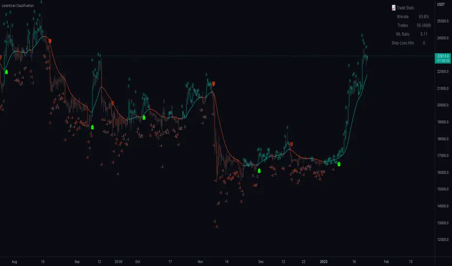
MLExtensionsLibrary "MLExtensions"
normalizeDeriv(src, quadraticMeanLength)
Returns the smoothed hyperbolic tangent of the input series.
Parameters:
src : The input series (i.e., the first-order derivative for price).
quadraticMeanLength : The length of the quadratic mean (RMS).
Returns: nDeriv The normalized derivative of the input series.
normalize(src, min, max)
Rescales a source value with an unbounded range to a target range.
Parameters:
src : The input series
min : The minimum value of the unbounded range
max : The maximum value of the unbounded range
Returns: The normalized series
rescale(src, oldMin, oldMax, newMin, newMax)
Rescales a source value with a bounded range to anther bounded range
Parameters:
src : The input series
oldMin : The minimum value of the range to rescale from
oldMax : The maximum value of the range to rescale from
newMin : The minimum value of the range to rescale to
newMax : The maximum value of the range to rescale to
Returns: The rescaled series
color_green(prediction)
Assigns varying shades of the color green based on the KNN classification
Parameters:
prediction : Value (int|float) of the prediction
Returns: color
color_red(prediction)
Assigns varying shades of the color red based on the KNN classification
Parameters:
prediction : Value of the prediction
Returns: color
tanh(src)
Returns the the hyperbolic tangent of the input series. The sigmoid-like hyperbolic tangent function is used to compress the input to a value between -1 and 1.
Parameters:
src : The input series (i.e., the normalized derivative).
Returns: tanh The hyperbolic tangent of the input series.
dualPoleFilter(src, lookback)
Returns the smoothed hyperbolic tangent of the input series.
Parameters:
src : The input series (i.e., the hyperbolic tangent).
lookback : The lookback window for the smoothing.
Returns: filter The smoothed hyperbolic tangent of the input series.
tanhTransform(src, smoothingFrequency, quadraticMeanLength)
Returns the tanh transform of the input series.
Parameters:
src : The input series (i.e., the result of the tanh calculation).
smoothingFrequency
quadraticMeanLength
Returns: signal The smoothed hyperbolic tangent transform of the input series.
n_rsi(src, n1, n2)
Returns the normalized RSI ideal for use in ML algorithms.
Parameters:
src : The input series (i.e., the result of the RSI calculation).
n1 : The length of the RSI.
n2 : The smoothing length of the RSI.
Returns: signal The normalized RSI.
n_cci(src, n1, n2)
Returns the normalized CCI ideal for use in ML algorithms.
Parameters:
src : The input series (i.e., the result of the CCI calculation).
n1 : The length of the CCI.
n2 : The smoothing length of the CCI.
Returns: signal The normalized CCI.
n_wt(src, n1, n2)
Returns the normalized WaveTrend Classic series ideal for use in ML algorithms.
Parameters:
src : The input series (i.e., the result of the WaveTrend Classic calculation).
n1
n2
Returns: signal The normalized WaveTrend Classic series.
n_adx(highSrc, lowSrc, closeSrc, n1)
Returns the normalized ADX ideal for use in ML algorithms.
Parameters:
highSrc : The input series for the high price.
lowSrc : The input series for the low price.
closeSrc : The input series for the close price.
n1 : The length of the ADX.
regime_filter(src, threshold, useRegimeFilter)
Parameters:
src
threshold
useRegimeFilter
filter_adx(src, length, adxThreshold, useAdxFilter)
filter_adx
Parameters:
src : The source series.
length : The length of the ADX.
adxThreshold : The ADX threshold.
useAdxFilter : Whether to use the ADX filter.
Returns: The ADX.
filter_volatility(minLength, maxLength, useVolatilityFilter)
filter_volatility
Parameters:
minLength : The minimum length of the ATR.
maxLength : The maximum length of the ATR.
useVolatilityFilter : Whether to use the volatility filter.
Returns: Boolean indicating whether or not to let the signal pass through the filter.
backtest(high, low, open, startLongTrade, endLongTrade, startShortTrade, endShortTrade, isStopLossHit, maxBarsBackIndex, thisBarIndex)
Performs a basic backtest using the specified parameters and conditions.
Parameters:
high : The input series for the high price.
low : The input series for the low price.
open : The input series for the open price.
startLongTrade : The series of conditions that indicate the start of a long trade.`
endLongTrade : The series of conditions that indicate the end of a long trade.
startShortTrade : The series of conditions that indicate the start of a short trade.
endShortTrade : The series of conditions that indicate the end of a short trade.
isStopLossHit : The stop loss hit indicator.
maxBarsBackIndex : The maximum number of bars to go back in the backtest.
thisBarIndex : The current bar index.
Returns: A tuple containing backtest values
init_table()
init_table()
Returns: tbl The backtest results.
update_table(tbl, tradeStatsHeader, totalTrades, totalWins, totalLosses, winLossRatio, winrate, stopLosses)
update_table(tbl, tradeStats)
Parameters:
tbl : The backtest results table.
tradeStatsHeader : The trade stats header.
totalTrades : The total number of trades.
totalWins : The total number of wins.
totalLosses : The total number of losses.
winLossRatio : The win loss ratio.
winrate : The winrate.
stopLosses : The total number of stop losses.
Returns: Updated backtest results table.

kNNLibrary "kNN"
Collection of experimental kNN functions. This is a work in progress, an improvement upon my original kNN script:
The script can be recreated with this library. Unlike the original script, that used multiple arrays, this has been reworked with the new Pine Script matrix features.
To make a kNN prediction, the following data should be supplied to the wrapper:
kNN : filter type. Right now either Binary or Percent . Binary works like in the original script: the system stores whether the price has increased (+1) or decreased (-1) since the previous knnStore event (called when either long or short condition is supplied). Percent works the same, but the values stored are the difference of prices in percents. That way larger differences in prices would give higher scores.
k : number k. This is how many nearest neighbors are to be selected (and summed up to get the result).
skew : kNN minimum difference. Normally, the prediction is done with a simple majority of the neighbor votes. If skew is given, then more than a simple majority is needed for a prediction. This also means that there are inputs for which no prediction would be given (if the majority votes are between -skew and +skew). Note that in Percent mode more profitable trades will have higher voting power.
depth : kNN matrix size limit. Originally, the whole available history of trades was used to make a prediction. This not only requires more computational power, but also neglects the fact that the market conditions are changing. This setting restricts the memory matrix to a finite number of past trades.
price : price series
long : long condition. True if the long conditions are met, but filters are not yet applied. For example, in my original script, trades are only made on crossings of fast and slow MAs. So, whenever it is possible to go long, this value is set true. False otherwise.
short : short condition. Same as long , but for short condition.
store : whether the inputs should be stored. Additional filters may be applied to prevent bad trades (for example, trend-based filters), so if you only need to consult kNN without storing the trade, this should be set to false.
feature1 : current value of feature 1. A feature in this case is some kind of data derived from the price. Different features may be used to analyse the price series. For example, oscillator values. Not all of them may be used for kNN prediction. As the current kNN implementation is 2-dimensional, only two features can be used.
feature2 : current value of feature 2.
The wrapper returns a tuple: [ longOK, shortOK ]. This is a pair of filters. When longOK is true, then kNN predicts a long trade may be taken. When shortOK is true, then kNN predicts a short trade may be taken. The kNN filters are returned whenever long or short conditions are met. The trade is supposed to happen when long or short conditions are met and when the kNN filter for the desired direction is true.
Exported functions :
knnStore(knn, p1, p2, src, maxrows)
Store the previous trade; buffer the current one until results are in. Results are binary: up/down
Parameters:
knn : knn matrix
p1 : feature 1 value
p2 : feature 2 value
src : current price
maxrows : limit the matrix size to this number of rows (0 of no limit)
Returns: modified knn matrix
knnStorePercent(knn, p1, p2, src, maxrows)
Store the previous trade; buffer the current one until results are in. Results are in percents
Parameters:
knn : knn matrix
p1 : feature 1 value
p2 : feature 2 value
src : current price
maxrows : limit the matrix size to this number of rows (0 of no limit)
Returns: modified knn matrix
knnGet(distance, result)
Get neighbours by getting k results with the smallest distances
Parameters:
distance : distance array
result : result array
Returns: array slice of k results
knnDistance(knn, p1, p2)
Create a distance array from the two given parameters
Parameters:
knn : knn matrix
p1 : feature 1 value
p2 : feature 2 value
Returns: distance array
knnSum(knn, p1, p2, k)
Make a prediction, finding k nearest neighbours and summing them up
Parameters:
knn : knn matrix
p1 : feature 1 value
p2 : feature 2 value
k : sum k nearest neighbors
Returns: sum of k nearest neighbors
doKNN(kNN, k, skew, depth, price, long, short, store, feature1, feature2)
execute kNN filter
Parameters:
kNN : filter type
k : number k
skew : kNN minimum difference
depth : kNN matrix size limit
price : series
long : long condition
short : short condition
store : store the supplied features (if false, only checks the results without storage)
feature1 : feature 1 value
feature2 : feature 2 value
Returns: filter output

Golden SlopeGolden Slope is an ATR based trend tool that mixes KNN machine learning to allow you to confirm your entry and exits, which can give out significantly more accurate signals.
Flag and rectangle signals are machine learning signals, they confirm an entry and exit position. You can use entry and exit signals alone but it's more accurate to confirm with machine learning signals. The idea is to either see a machine learning signal first and confirm it by Golden Slope entry or the other way around.
PS. Watch out if candle starts hitting the golden belly (or the yellow area after an entry signal is given because it can indicate a reversal before machine learning or the golden slope itself catch it, but these events happen rarely.

Machine Learning: kNN (New Approach)Description:
kNN is a very robust and simple method for data classification and prediction. It is very effective if the training data is large. However, it is distinguished by difficulty at determining its main parameter, K (a number of nearest neighbors), beforehand. The computation cost is also quite high because we need to compute distance of each instance to all training samples. Nevertheless, in algorithmic trading KNN is reported to perform on a par with such techniques as SVM and Random Forest. It is also widely used in the area of data science.
The input data is just a long series of prices over time without any particular features. The value to be predicted is just the next bar's price. The way that this problem is solved for both nearest neighbor techniques and for some other types of prediction algorithms is to create training records by taking, for instance, 10 consecutive prices and using the first 9 as predictor values and the 10th as the prediction value. Doing this way, given 100 data points in your time series you could create 10 different training records. It's possible to create even more training records than 10 by creating a new record starting at every data point. For instance, you could take the first 10 data points and create a record. Then you could take the 10 consecutive data points starting at the second data point, the 10 consecutive data points starting at the third data point, etc.
By default, shown are only 10 initial data points as predictor values and the 6th as the prediction value.
Here is a step-by-step workthrough on how to compute K nearest neighbors (KNN) algorithm for quantitative data:
1. Determine parameter K = number of nearest neighbors.
2. Calculate the distance between the instance and all the training samples. As we are dealing with one-dimensional distance, we simply take absolute value from the instance to value of x (| x – v |).
3. Rank the distance and determine nearest neighbors based on the K'th minimum distance.
4. Gather the values of the nearest neighbors.
5. Use average of nearest neighbors as the prediction value of the instance.
The original logic of the algorithm was slightly modified, and as a result at approx. N=17 the resulting curve nicely approximates that of the sma(20). See the description below. Beside the sma-like MA this algorithm also gives you a hint on the direction of the next bar move.

Machine Learning & Optimization Moving Average (Expo)█ An indicator that finds the best moving average
We all know that the market change in characteristics over time, volatility, volume, momentum, etc., keep changing. Therefore, traders fine-tune their indicators and strategies to fit the constantly changing market. Unfortunately, that means there is no "best" MA period that suits all these conditions. That is why we have developed this algorithm that self-adapts and finds the best MA period based on Machine Learning and Optimization calculations.
This indicator help traders and investors to use the best possible moving average period on the selected timeframe and asset and ensures that the period is updated even though the market characteristics change over time.
█ Self-optimizing moving average
There is no doubt that different markets and timeframes need different MA periods. Therefore, our algorithm optimizes the moving average period within the given parameter range and optimizes its value based on either performance, win rate, or the combined results. The moving average period updates automatically on the chart for you.
Traders can choose to use our Machine Learning Algorithm to optimize the MA values or can optimize only using the optimization algorithm.
Performance
If you select to optimize based on performance, the calculation returns the period with the highest gains.
Winrate
If you select to optimize based on win rate, the calculation returns the period that gives the best win rate.
Combined
If you select to optimize based on combined results, the calculations score the performance and win rate separately and choose the best period with the highest ranking in both aspects.
█ Finding the best moving average for any asset and timeframe
Traders can choose to find the best moving average based on price crossings.
█ Finding the best combination of moving averages for any asset and timeframe
Traders can choose to find the best crossing strategy, where the algorithm compares the 2 averages and returns the best fast and slow period.
█ Alerts
Traders can choose to be alerted when a new best moving average is found or when a moving average cross occurs.
-----------------
Disclaimer
The information contained in my Scripts/Indicators/Ideas/Algos/Systems does not constitute financial advice or a solicitation to buy or sell any securities of any type. I will not accept liability for any loss or damage, including without limitation any loss of profit, which may arise directly or indirectly from the use of or reliance on such information.
All investments involve risk, and the past performance of a security, industry, sector, market, financial product, trading strategy, backtest, or individual's trading does not guarantee future results or returns. Investors are fully responsible for any investment decisions they make. Such decisions should be based solely on an evaluation of their financial circumstances, investment objectives, risk tolerance, and liquidity needs.
My Scripts/Indicators/Ideas/Algos/Systems are only for educational purposes!

Esqvair's Neural Reversal Probability IndicatorIntroduction
Esqvair's Neural Reversal Probability Indicator is the indicator that shows probability of reversal.
Warning: This script should only be used on 1 minute chart.
How to use
When a signal appears (by default it is a green bar), a reversal should be expected.
The signal appears when the indicator value >= Threshold.
If you want more signals, you must lower the threshold, if less, you must increase the threshold.
For some assets, like Forex pairs, you have to optimize the threshold yourself, but for most stocks, the default threshold works well.
How well a threshold fits an asset depends on the volatility of the asset.
For most assets, the indicator ranges from 35 to 75.
Settings
Smoothing - The default is 1, which means no smoothing. Indicator smoothing by SMA.
Threshold - default 71.0 is responsible for the occurrence of signals, read "How to use" part to learn more
The Indicator
This indicator is a pre-trained neural network that was trained outside of TradingView and then its structure and weights values were converted to PineScript.
Warning: A neural network is a black box in the sense that although it can approximate any function, studying its structure will not give you any idea about the structure of the function being approximated.
Possible questions
Why does the indicator value most time range from 35 to 75 when the probability should ranges from 0 to 100?
-Due to some randomness in the markets, a neural network can never be 100% sure.
What data was used to train the neural network?
-This was BTCUSD 1 minute chart data from 02/05/2020 to 02/05/2022.
Where did you train the neural network and convert it to PineScript?
-I used a programming language that I know.
