Universal Moving Average🙏🏻 UMA (Universal Moving Average) represents the most natural and prolly ‘the’ final general universal entity for calculating rolling typical value for any type of time-series. Simply via different weighting schemes applied together, it encodes:
Location of each datapoint in corresponding fields (price, time, volume)
Informational relevance of each datapoint via using windowing functions that are fundamental in nature and go beyond DSP inventions & approximations
Innovation in state space (in our case = volatility)
The real beauty of this development: being simply a weighting scheme that can be applied to anything: be it weighted median , weighted quantile regression, or weighted KDE , or a simple weighted mean (like in this script). As long as a method accepts weights, you can harness the power of this entity. It means that final algorithmic complexity will match your initial tool.
As a moving ‘average’ it beats ALMA, KAMA, MAMA, VIDYA and all others because it is a simple and general entity, and all it does is encoding ‘all’ available information. I think that post might anger a lot of people, because lotta things will be realized as legacy and many paywalls gonna be ignored, specially for the followers of DSP cult, the ones who yet don’t understand that aggregated tick data is not a signal omg, it’s a completely different type of time series where your methods simply don’t fit even closely. I am also sorry to inform y’all, that spectral analysis is much closer to state-space methods in spirit than to DSP. But in fact DSP is cool and I love it, well for actual signals xD
...
Weights explained & how to use them: as I already said, the whole thing is based on combining different set of weights, and you can turn them on/off in script settings. Btw I've set em up defaults so you can use the thing on price data out of the box right away.
Price, Time, Volume weights: encode location of every datapoint in Price & TIme & Volume field
Howtouse: u have to disable one weight that corresponds to the field you apply UMA to. E.g if you apply UMA to prices, you turn off price weighting And turn on time and volume weighting. Or if you apply UMA to volume delta, you turn off volume weighting And turn on price and time weighting.
Higher prices are more important, this asymmetry is confirmed and even proved by the fact that prices can’t be negative (don’t even mention that incorrect rollover on CL contract in 2k20...).
Signal weights: encode actuality/importance/relevance of datapoints.
Howtouse: in DSP terms, it provides smoothing, but also compensates for the lag it introduces. This smoothness is useful if you use slope reversals for signal generation aka watching peaks and valleys in a moving average shape. It's also better to perturb smoothed outputs with this , this way you inject high freq content back, But in controlled way!
Signal = information.
The fundamental universal entity behind so-called “smoothing” in DSP has nothing to do with signals and goes eons beyond DSP. This is simply about measuring the relevance of data in time.
First, new datapoints need some time to be “embedded” into the timeline, you can think of it as time proof, kinda stuff needs time to be proved, accepted; while earliest datapoints lose relevance in time.
Second, along with the first notion, at the same time there’s the counter notion that simply weights new data more, acting as a counterweight from the down-weighting of the latest datapoints introduced by the first notion.
The first part can be represented as PDF of beta(2, 2) window (a set of weights in our case). It’s actually well known as the Welch window, that lives in between so called statistical and DSP worlds, emerges in multiple contexts. Mainstream DSP users tho mostly don’t use this one, they use primitive legacy windowing function, you can find all kinds on this wiki page.
Now the second part, where DSP adepts usually stop, is to introduce the second compensating windowing function. Instead they try to reduce window size, or introduce other kinds of volatility weights, do some tricks, but it ain’t provides obviously. The natural step here is to simply use the integral of the initial window; if the initial window is beta(2, 2) then what we simply need is CDF of beta(2, 2), in fact the vertically inverted shape of it aka survival function . That’s it bros. Simply as that.
When both of these are applied you have smth magical, your output becomes smooth and yet not lagging. No arbitrary windowing functions, tricks with data modification etc
Why beta(2, 2)? It naturally arises in many contexts, it’s based on one of the most fundamental functions in the universe: x^2. It has finite support. I can talk more bout it on request, but I am absolutely sure this is it.
^^ impulse response of the resulting weighs together (green) compared with uniform weights aka boxcar (red). Made with this script .
Weighing by state: encodes state-space innovation of each datapoint, basically magnitude of changes, strength of these changes, aka volatility.
Howtouse: this makes your moving average volatility aware in proper math ways. The influence of datapoints will be stronger when changes are stronger. This is weighting by innovations, or weighting by volatility by using squared returns.
Why squared returns? They encode state‑space innovations properly because the innovation of any continuous‑time semimartingale is about its quadratic variation, and quadratic variation is built from squared increments, not absolute increments.
Adaptive length is not the right way to introduce adaptivity by volatility xD. When you weight datapoints by squared returns you’re already dynamically varying ‘effective’ data size, you don’t need anything else.
...
It’s all good, progress happens, that’s how the Universe works, that's how Universal Moving Average works. Time to evolve. I might update other scripts with this complete weighting scheme, either by my own desire or your request.
...
∞
Returns

Macro Return ForecastWhen the macro environment was similar, what annualized return did the market usually deliver next?
Before using the indicator, make sure your chart is set to any US-market symbol (SPX, QQQ, DIA, etc.).
This requirement is simple: the indicator pulls macro series from US data (yields, TIPS, credit spreads, breadth of US indices).
Because these series are independent from the chart’s price series, the chart symbol itself does not affect the internal calculations.
Any US symbol works, and the output of the model will be identical as long as you are on a US asset with daily, weekly or monthly timeframe.
The plotted price does not matter: the macro engine is fully exogenous to the chart symbol.
1. What the indicator does relative to selected assets
In the settings you choose which market you want to analyze:
- S&P500
- Nasdaq or NQ100
- Dow Jones
- Russell 2000
- US-wide (VTI)
- S&P500 sectors (XLF, XLY, XLP, etc.)
For each one, the indicator loads:
- Its internal breadth series (percentage of constituents above MA200)
- Its price history to compute forward log-returns at multiple horizons
- Its regime position relative to its own MA200 (for bull/bear filtering)
This means the tool is not tied to the chart symbol you display.
If your chart is SPX but the indicator setting is “S&P500 Technology”, the expected return projection is computed for the Technology sector using its own data, not the chart’s data.
You can therefore:
- Visualize macro-driven expected returns for any major US index or sector.
- Compare how different parts of the market historically reacted to similar macro states.
- Switch assets instantly to see which segment historically behaved better in comparable macro conditions.
The indicator becomes an analyzer of macro sensitivity, not a chart-dependent indicator.
2. Method overview
The model answers a statistical question:
“When macro conditions looked like they do today, what forward annualized return did this asset usually deliver?”
To do this it combines four macro pillars:
- Market breadth of the selected asset
- Yield curve slope (US 10Y minus 2Y)
- US credit spread (high yield minus gov)
- US real rate (TIPS 10Y)
It normalizes each metric into a 0–100 score, groups similar historical states into bins, and examines what the asset did next across six horizons (from ~9 months to ~5 years).
This produces a historical map connecting macro states to realized forward returns.
It is not a forecast model.
It is a conditional-distribution estimator: it tells you what has historically happened from similar setups.
3. Why this produces useful insights on assets
For any chosen asset (SPX, Nasdaq, sectors…), the indicator computes:
- Its forward return distribution in similar macro states.
- How often these states occurred (n).
- Whether the macro environment that preceded positive returns in the past resembles today’s.
- Whether the asset tends to be more sensitive or more resilient than the broad index under given macro configurations.
- Whether a given sector historically benefited from specific yield-curve, credit or real-rate environments.
This lets you answer questions such as:
- Does this sector usually outperform in an inverted yield curve environment?
- Does the Nasdaq historically recover strongly after breadth collapses?
- How did the S&P500 behave historically when real rates were this high?
- Is today’s credit-spread environment typically associated with positive or negative forward returns for this index?
These insights are not predictions but statistical context backed by past market behavior.
4. Why the technique is robust (and why it matters)
The engine uses strict, non-optimistic data processing:
- Winsorization of returns to neutralize extreme outliers without deleting information.
- Shrinkage estimators to avoid overfitting when bins contain few occurrences.
- Adaptive or static bounds for scaling macro indicators, ensuring comparability across cycles.
- Inverse-variance weighting of horizons with penalties for horizon redundancy.
- HAC-style adjustments to reduce autocorrelation bias in return estimation.
Each method aims to prevent artificial inflation of expected-return values and to keep the estimator stable even in unusual macro states.
This produces a result that is not “optimistic”, not curve-fit, not dependent on chart tricks, and not sensitive to isolated historical anomalies.
5. What you get as a user
A single clean line:
Expected Annual Return (%)
This line reflects how the chosen asset historically performed after macro environments similar to today’s.
The color gradient and confidence indicator (n) show the density of comparable episodes in history.
This makes the output extremely simple to read:
- High, stable expectation: historically supportive macro environment.
- Low or negative expectation: historically weaker environments.
- Low confidence: the macro state is rare and historical comparisons are limited.
The tool therefore adds context, not signals.
It helps you understand the environment the asset is currently in, based on how markets behaved in similar conditions across US market history.

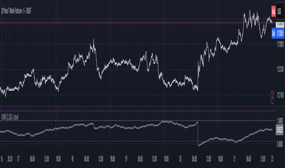
Volatility Signal-to-Noise Ratio🙏🏻 this is VSNR: the most effective and simple volatility regime detector & automatic volatility threshold scaler that somehow no1 ever talks about.
This is simply an inverse of the coefficient of variation of absolute returns, but properly constructed taking into account temporal information, and made online via recursive math with algocomplexity O(1) both in expanding and moving windows modes.
How do the available alternatives differ (while some’re just worse)?
Mainstream quant stat tests like Durbin-Watson, Dickey-Fuller etc: default implementations are ALL not time aware. They measure different kinds of regime, which is less (if at all) relevant for actual trading context. Mix of different math, high algocomplexity.
The closest one is MMI by financialhacker, but his approach is also not time aware, and has a higher algocomplexity anyways. Best alternative to mine, but pls modify it to use a time-weighted median.
Fractal dimension & its derivatives by John Ehlers: again not time aware, very low info gain, relies on bar sizes (high and lows), which don’t always exist unlike changes between datapoints. But it’s a geometric tool in essence, so this is fundamental. Let it watch your back if you already use it.
Hurst exponent: much higher algocomplexity, mix of parametric and non-parametric math inside. An invention, not a math entity. Again, not time aware. Also measures different kinds of regime.
How to set it up:
Given my other tools, I choose length so that it will match the amount of data that your trading method or study uses multiplied by ~ 4-5. E.g if you use some kind of bands to trade volatility and you calculate them over moving window 64, put VSNR on 256.
However it depends mathematically on many things, so for your methods you may instead need multipliers of 1 or ~ 16.
Additionally if you wanna use all data to estimate SNR, put 0 into length input.
How to use for regime detection:
First we define:
MR bias: mean reversion bias meaning volatility shorts would work better, fading levels would work better
Momo bias: momentum bias meaning volatility longs would work better, trading breakouts of levels would work better.
The study plots 3 horizontal thresholds for VSNR, just check its location:
Above upper level: significant Momo bias
Above 1 : Momo bias
Below 1 : MR bias
Below lower level: significant MR bias
Take a look at the screenshots, 2 completely different volatility regimes are spotted by VSNR, while an ADF does not show different regime:
^^ CBOT:ZN1!
^^ INDEX:BTCUSD
How to use as automatic volatility threshold scaler
Copy the code from the script, and use VSNR as a multiplier for your volatility threshold.
E.g you use a regression channel and fade/push upper and lower thresholds which are RMSEs multiples. Inside the code, multiply RMSE by VSNR, now you’re adaptive.
^^ The same logic as when MM bots widen spreads with vola goes wild.
How it works:
Returns follow Laplace distro -> logically abs returns follow exponential distro , cuz laplace = double exponential.
Exponential distro has a natural coefficient of variation = 1 -> signal to noise ratio defined as mean/stdev = 1 as well. The same can be said for Student t distro with parameter v = 4. So 1 is our main threshold.
We can add additional thresholds by discovering SNRs of Student t with v = 3 and v = 5 (+- 1 from baseline v = 4). These have lighter & heavier tails each favoring mean reversion or momentum more. I computed the SNR values you see in the code with mpmath python module, with precision 256 decimals, so you can trust it I put it on my momma.
Then I use exponential smoothing with properly defined alphas (one matches cumulative WMA and another minimizes error with WMA in moving window mode) to estimate SNR of abs returns.
…
Lightweight huh?
∞
Market Breadth & Forward ReturnsThis indicator shows how future index performance has historically behaved after different levels of market breadth. The heatmap reveals which breadth zones have tended to precede better or worse forward returns. This is strictly a statistical conditional-expectation map, not a set of signals.
Scope
This is not meant for any arbitrary asset.
It is meant for broad indices only (S&P 500, Nasdaq 100, Dow, Russell, major sector families).
The breadth data is derived from index-level market universes.
Do not apply this on single stocks, crypto or FX. The method only makes sense with large diversified universes.
Core method
Daily breadth is normalized 0 to 100.
For each bar, six forward horizons are evaluated on the index: performance after X days.
Each observation is placed into a breadth bin.
Each bin/horizon pair has mean, variance and count computed.
Each bin/horizon mean is t-tested against zero.
Benjamini-Hochberg False Discovery Rate weighting allocates weight only to horizons where evidence exists.
Weighted horizon means are aggregated and annualized (252 trading days).
The map displays annualized conditional forward returns per breadth bin.
Why this is robust
Non-repainting. Breadth is in the past, returns are strictly future, lookahead_off.
Multiple horizons avoid single-window biases.
Variance, t-tests and FDR correction drastically reduce false positives.
Bins with poor sample size are visually suppressed to avoid over-interpretation.
How to use
Daily timeframe only.
Select the correct index family (S&P 500, Nasdaq 100, Russell…).
Bin size 5 to 10 points is a realistic range.
Min occurrences per bin ≥ 5 recommended.
FDR alpha 0.05 to 0.10 is a good working envelope.
Interpret as conditional expectations, not a forecast guarantee.
Notes
Do not use on random assets.
Do not extrapolate outside the chosen index family.
Always keep symbol and timeframe visible when publishing.
Indicator by Julien Eche

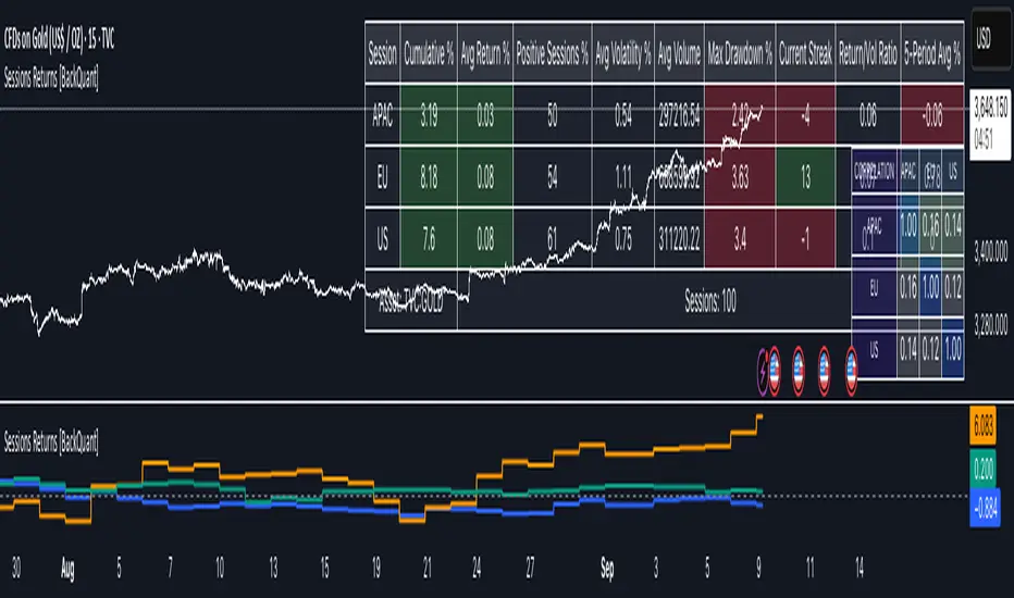
Cumulative Returns by Session [BackQuant]Cumulative Returns by Session
What this is
This tool breaks the trading day into three user-defined sessions and tracks how much each session contributes to return, volatility, and volume. It then aggregates results over a rolling window so you can see which session has been pulling its weight, how streaky each session has been, and how sessions relate to one another through a compact correlation heatmap.
We’ve also given the functionality for the user to use a simplified table, just by switching off all settings they are not interested in.
How it works
1) Session segmentation
You define APAC, EU, and US sessions with explicit hours and time zones. The script detects when each session starts and ends on every intraday bar and records its open, intraday high and low, close, and summed volume.
2) Per-session math
At each session end the script computes:
Return — either Percent: (Close−Open)÷Open×100(Close − Open) ÷ Open × 100(Close−Open)÷Open×100 or Points: (Close−Open)(Close − Open)(Close−Open), based on your selection.
Volatility — either Range: (High−Low)÷Open×100(High − Low) ÷ Open × 100(High−Low)÷Open×100 or ATR scaled by price: ATR÷Open×100ATR ÷ Open × 100ATR÷Open×100.
Volume — total volume transacted during that session.
3) Storage and lookback
Each day’s three session stats are stored as a row. You choose how many recent sessions to keep in memory. The script then:
Builds cumulative returns for APAC, EU, US across the lookback.
Computes averages, win rates, and a Sharpe-like ratio avgreturn÷avgvolatilityavg return ÷ avg volatilityavgreturn÷avgvolatility per session.
Tracks streaks of positive or negative sessions to show momentum.
Tracks drawdowns on cumulative returns to show worst runs from peak.
Computes rolling means over a short window for short-term drift.
4) Correlation heatmap
Using the stored arrays of session returns, the script calculates Pearson correlations between APAC–EU, APAC–US, and EU–US, and colors the matrix by strength and sign so you can spot coupling or decoupling at a glance.
What it plots
Three lines: cumulative return for APAC, EU, US over the chosen lookback.
Zero reference line for orientation.
A statistics table with cumulative %, average %, positive session rate, and optional columns for volatility, average volume, max drawdown, current streak, return-to-vol ratio, and rolling average.
A small correlation heatmap table showing APAC, EU, US cross-session correlations.
How to use it
Pick the asset — leave Custom Instrument empty to use the chart symbol, or point to another symbol for cross-asset studies.
Set your sessions and time zones — defaults approximate APAC, EU, and US hours, but you can align them to exchange times or your workflow.
Choose calculation modes — Percent vs Points for return, Range vs ATR for volatility. Points are convenient for futures and fixed-tick assets, Percent is comparable across symbols.
Decide the lookback — more sessions smooths lines and stats; fewer sessions makes the tool more reactive.
Toggle analytics — add volatility, volume, drawdown, streaks, Sharpe-like ratio, rolling averages, and the correlation table as needed.
Why session attribution helps
Different sessions are driven by different flows. Asia often sets the overnight tone, Europe adds liquidity and direction changes, and the US session can dominate range expansion. Separating contributions by session helps you:
Identify which session has been the main driver of net trend.
Measure whether volatility or volume is concentrated in a specific window.
See if one session’s gains are consistently given back in another.
Adapt tactics: fade during a mean-reverting session, press during a trending session.
Reading the tables
Cumulative % — sum of session returns over the lookback. The sign and slope tell you who is carrying the move.
Avg Return % and Positive Sessions % — direction and hit rate. A low average but high hit rate implies many small moves; the reverse implies occasional big swings.
Avg Volatility % — typical intrabars range for that session. Compare with Avg Return to judge efficiency.
Return/Vol Ratio — return per unit of volatility. Higher is better for stability.
Max Drawdown % — worst cumulative give-back within the lookback. A quick way to spot riskiness by session.
Current Streak — consecutive up or down sessions. Useful for mean-reversion or regime awareness.
Rolling Avg % — short-window drift indicator to catch recent turnarounds.
Correlation matrix — green clusters indicate sessions tending to move together; red indicates offsetting behavior.
Settings overview
Basic
Number of Sessions — how many recent days to include.
Custom Instrument — analyze another ticker while staying on your current chart.
Session Configuration and Times
Enable or hide APAC, EU, US rows.
Set hours per session and the specific time zone for each.
Calculation Methods
Return Calculation — Percent or Points.
Volatility Calculation — Range or ATR; ATR Length when applicable.
Advanced Analytics
Correlation, Drawdown, Momentum, Sharpe-like ratio, Rolling Statistics, Rolling Period.
Display Options and Colors
Show Statistics Table and its position.
Toggle columns for Volatility and Volume.
Pick individual colors for each session line and row accents.
Common applications
Session bias mapping — find which window tends to trend in your market and plan exposure accordingly.
Strategy scheduling — allocate attention or risk to the session with the best return-to-vol ratio.
News and macro awareness — see if correlation rises around central bank cycles or major data releases.
Cross-asset monitoring — set the Custom Instrument to a driver (index future, DXY, yields) to see if your symbol reacts in a particular session.
Notes
This indicator works on intraday charts, since sessions are defined within a day. If you change session clocks or time zones, give the script a few bars to accumulate fresh rows. Percent vs Points and Range vs ATR choices affect comparability across assets, so be consistent when comparing symbols.
Session context is one of the simplest ways to explain a messy tape. By separating the day into three windows and scoring each one on return, volatility, and consistency, this tool shows not just where price ended up but when and how it got there. Use the cumulative lines to spot the steady driver, read the table to judge quality and risk, and glance at the heatmap to learn whether the sessions are amplifying or canceling one another. Adjust the hours to your market and let the data tell you which session deserves your focus.
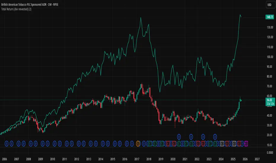
Total Return (divi reivested)Total Return (Dividends Reinvested) — Price Scale
This indicator overlays a Total Return price line on the chart. It shows how the stock would have performed if all dividends had been reinvested back into the stock (buying fractional shares) rather than taken as cash.
The line starts exactly at the price level of the first visible bar on your chart and moves in the same price units as the chart (not indexed to 100).
Until the first dividend inside the visible window, the Total Return line is identical to the price. From the first dividend onward, it gradually diverges upwards, reflecting the effect of reinvested payouts.
Settings:
Reinvest at Open / Close — Choose whether reinvestment uses the bar’s open or close price.
Apply effect on the next bar — If enabled, reinvestment shows up from the bar after the dividend date (common in practice).
Show dividend markers — Optionally plots labels where dividend events occur.
Line width — Adjusts the thickness of the plotted Total Return line.
Use case:
This tool is useful if you want to compare plain price performance with true shareholder returns including dividends. It helps evaluate dividend stocks (like BTI, T, XOM, etc.) more realistically.
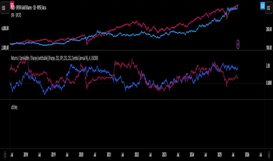
Rolling Performance Toolkit (Returns, Correlation and Sharpe)This script provides a flexible toolkit for evaluating rolling performance metrics between any asset and a benchmark.
Features:
Library-based: Built on a custom utilities library for consistent return and statistics calculations.
Rolling Window Control: Choose the lookback period (in days) to calculate metrics.
Multiple Modes: Toggle between Rolling Returns, Rolling Correlation, and Rolling Sharpe Ratio.
Benchmark Comparison: Compare your selected ticker against a benchmark (default: S&P 500 / SPX), but you can easily switch to any symbol.
Risk-Free Rate Options: Choose from zero, a constant annual % rate, or a proxy symbol (default: US03M – 3-Month Treasury Yield).
Annualized Sharpe: Sharpe ratios are annualized by default (×√252) for intuitive interpretation.
This tool is useful for traders and investors who want to monitor relative performance, diversification benefits, or risk-adjusted returns over time.
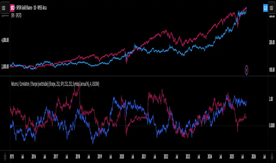
utilitiesLibrary for commonly used utilities, for visualizing rolling returns, correlations and sharpe
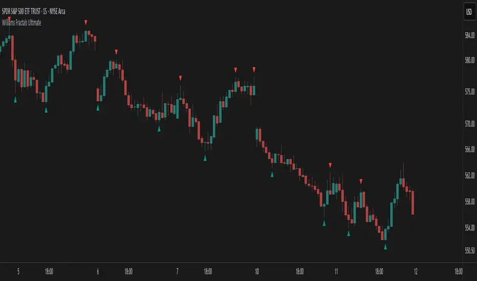
Williams Fractals Ultimate (Donchian Adjusted)Williams Fractals Ultimate (Donchian Adjusted)
Understanding Williams Fractals
Williams Fractals are a simple yet powerful tool used to identify potential turning points in the market. They highlight local highs (up fractals) and local lows (down fractals) based on a set period.
An up fractal appears when a price peak is higher than the surrounding prices.
A down fractal appears when a price low is lower than the surrounding prices.
Fractals help traders spot support and resistance levels, potential trend reversals, and price breakout zones.
Why Adjust Fractals with the Donchian Channel?
The standard Williams Fractals method identifies local highs and lows without considering broader market context. This script enhances fractal accuracy by integrating the Donchian Channel, which tracks the highest highs and lowest lows over a set period.
- The Donchian Baseline is calculated as the average of the highest high and lowest low over a selected period.
- Fractals are filtered based on this baseline:
Up Fractals are only shown if they are above the Donchian baseline.
Down Fractals are only shown if they are below the Donchian baseline.
This filtering method removes weak signals and ensures that only relevant fractals aligned with market structure are displayed.
Key Features of the Script
Customizable Fractal & Donchian Periods – Allows traders to fine-tune fractal sensitivity.
Donchian-Based Filtering – Reduces noise and highlights meaningful fractals.
Fractal ZigZag Line (Optional) – Helps visualize price swings more clearly.
Why Is This So Effective?
Stronger trend signals – Filtering with the Donchian baseline eliminates unreliable fractals.
Clearer price action – The optional ZigZag line visually connects significant highs and lows.
Easy trend identification – Helps traders confirm breakout zones and key price levels.
This script is a technical analysis tool and does not guarantee profitable trades. Always combine it with other indicators and risk management strategies before making trading decisions.
ValueAtTime█ OVERVIEW
This library is a Pine Script® programming tool for accessing historical values in a time series using UNIX timestamps . Its data structure and functions index values by time, allowing scripts to retrieve past values based on absolute timestamps or relative time offsets instead of relying on bar index offsets.
█ CONCEPTS
UNIX timestamps
In Pine Script®, a UNIX timestamp is an integer representing the number of milliseconds elapsed since January 1, 1970, at 00:00:00 UTC (the UNIX Epoch ). The timestamp is a unique, absolute representation of a specific point in time. Unlike a calendar date and time, a UNIX timestamp's meaning does not change relative to any time zone .
This library's functions process series values and corresponding UNIX timestamps in pairs , offering a simplified way to identify values that occur at or near distinct points in time instead of on specific bars.
Storing and retrieving time-value pairs
This library's `Data` type defines the structure for collecting time and value information in pairs. Objects of the `Data` type contain the following two fields:
• `times` – An array of "int" UNIX timestamps for each recorded value.
• `values` – An array of "float" values for each saved timestamp.
Each index in both arrays refers to a specific time-value pair. For instance, the `times` and `values` elements at index 0 represent the first saved timestamp and corresponding value. The library functions that maintain `Data` objects queue up to one time-value pair per bar into the object's arrays, where the saved timestamp represents the bar's opening time .
Because the `times` array contains a distinct UNIX timestamp for each item in the `values` array, it serves as a custom mapping for retrieving saved values. All the library functions that return information from a `Data` object use this simple two-step process to identify a value based on time:
1. Perform a binary search on the `times` array to find the earliest saved timestamp closest to the specified time or offset and get the element's index.
2. Access the element from the `values` array at the retrieved index, returning the stored value corresponding to the found timestamp.
Value search methods
There are several techniques programmers can use to identify historical values from corresponding timestamps. This library's functions include three different search methods to locate and retrieve values based on absolute times or relative time offsets:
Timestamp search
Find the value with the earliest saved timestamp closest to a specified timestamp.
Millisecond offset search
Find the value with the earliest saved timestamp closest to a specified number of milliseconds behind the current bar's opening time. This search method provides a time-based alternative to retrieving historical values at specific bar offsets.
Period offset search
Locate the value with the earliest saved timestamp closest to a defined period offset behind the current bar's opening time. The function calculates the span of the offset based on a period string . The "string" must contain one of the following unit tokens:
• "D" for days
• "W" for weeks
• "M" for months
• "Y" for years
• "YTD" for year-to-date, meaning the time elapsed since the beginning of the bar's opening year in the exchange time zone.
The period string can include a multiplier prefix for all supported units except "YTD" (e.g., "2W" for two weeks).
Note that the precise span covered by the "M", "Y", and "YTD" units varies across time. The "1M" period can cover 28, 29, 30, or 31 days, depending on the bar's opening month and year in the exchange time zone. The "1Y" period covers 365 or 366 days, depending on leap years. The "YTD" period's span changes with each new bar, because it always measures the time from the start of the current bar's opening year.
█ CALCULATIONS AND USE
This library's functions offer a flexible, structured approach to retrieving historical values at or near specific timestamps, millisecond offsets, or period offsets for different analytical needs.
See below for explanations of the exported functions and how to use them.
Retrieving single values
The library includes three functions that retrieve a single stored value using timestamp, millisecond offset, or period offset search methods:
• `valueAtTime()` – Locates the saved value with the earliest timestamp closest to a specified timestamp.
• `valueAtTimeOffset()` – Finds the saved value with the earliest timestamp closest to the specified number of milliseconds behind the current bar's opening time.
• `valueAtPeriodOffset()` – Finds the saved value with the earliest timestamp closest to the period-based offset behind the current bar's opening time.
Each function has two overloads for advanced and simple use cases. The first overload searches for a value in a user-specified `Data` object created by the `collectData()` function (see below). It returns a tuple containing the found value and the corresponding timestamp.
The second overload maintains a `Data` object internally to store and retrieve values for a specified `source` series. This overload returns a tuple containing the historical `source` value, the corresponding timestamp, and the current bar's `source` value, making it helpful for comparing past and present values from requested contexts.
Retrieving multiple values
The library includes the following functions to retrieve values from multiple historical points in time, facilitating calculations and comparisons with values retrieved across several intervals:
• `getDataAtTimes()` – Locates a past `source` value for each item in a `timestamps` array. Each retrieved value's timestamp represents the earliest time closest to one of the specified timestamps.
• `getDataAtTimeOffsets()` – Finds a past `source` value for each item in a `timeOffsets` array. Each retrieved value's timestamp represents the earliest time closest to one of the specified millisecond offsets behind the current bar's opening time.
• `getDataAtPeriodOffsets()` – Finds a past value for each item in a `periods` array. Each retrieved value's timestamp represents the earliest time closest to one of the specified period offsets behind the current bar's opening time.
Each function returns a tuple with arrays containing the found `source` values and their corresponding timestamps. In addition, the tuple includes the current `source` value and the symbol's description, which also makes these functions helpful for multi-interval comparisons using data from requested contexts.
Processing period inputs
When writing scripts that retrieve historical values based on several user-specified period offsets, the most concise approach is to create a single text input that allows users to list each period, then process the "string" list into an array for use in the `getDataAtPeriodOffsets()` function.
This library includes a `getArrayFromString()` function to provide a simple way to process strings containing comma-separated lists of periods. The function splits the specified `str` by its commas and returns an array containing every non-empty item in the list with surrounding whitespaces removed. View the example code to see how we use this function to process the value of a text area input .
Calculating period offset times
Because the exact amount of time covered by a specified period offset can vary, it is often helpful to verify the resulting times when using the `valueAtPeriodOffset()` or `getDataAtPeriodOffsets()` functions to ensure the calculations work as intended for your use case.
The library's `periodToTimestamp()` function calculates an offset timestamp from a given period and reference time. With this function, programmers can verify the time offsets in a period-based data search and use the calculated offset times in additional operations.
For periods with "D" or "W" units, the function calculates the time offset based on the absolute number of milliseconds the period covers (e.g., `86400000` for "1D"). For periods with "M", "Y", or "YTD" units, the function calculates an offset time based on the reference time's calendar date in the exchange time zone.
Collecting data
All the `getDataAt*()` functions, and the second overloads of the `valueAt*()` functions, collect and maintain data internally, meaning scripts do not require a separate `Data` object when using them. However, the first overloads of the `valueAt*()` functions do not collect data, because they retrieve values from a user-specified `Data` object.
For cases where a script requires a separate `Data` object for use with these overloads or other custom routines, this library exports the `collectData()` function. This function queues each bar's `source` value and opening timestamp into a `Data` object and returns the object's ID.
This function is particularly useful when searching for values from a specific series more than once. For instance, instead of using multiple calls to the second overloads of `valueAt*()` functions with the same `source` argument, programmers can call `collectData()` to store each bar's `source` and opening timestamp, then use the returned `Data` object's ID in calls to the first `valueAt*()` overloads to reduce memory usage.
The `collectData()` function and all the functions that collect data internally include two optional parameters for limiting the saved time-value pairs to a sliding window: `timeOffsetLimit` and `timeframeLimit`. When either has a non-na argument, the function restricts the collected data to the maximum number of recent bars covered by the specified millisecond- and timeframe-based intervals.
NOTE : All calls to the functions that collect data for a `source` series can execute up to once per bar or realtime tick, because each stored value requires a unique corresponding timestamp. Therefore, scripts cannot call these functions iteratively within a loop . If a call to these functions executes more than once inside a loop's scope, it causes a runtime error.
█ EXAMPLE CODE
The example code at the end of the script demonstrates one possible use case for this library's functions. The code retrieves historical price data at user-specified period offsets, calculates price returns for each period from the retrieved data, and then populates a table with the results.
The example code's process is as follows:
1. Input a list of periods – The user specifies a comma-separated list of period strings in the script's "Period list" input (e.g., "1W, 1M, 3M, 1Y, YTD"). Each item in the input list represents a period offset from the latest bar's opening time.
2. Process the period list – The example calls `getArrayFromString()` on the first bar to split the input list by its commas and construct an array of period strings.
3. Request historical data – The code uses a call to `getDataAtPeriodOffsets()` as the `expression` argument in a request.security() call to retrieve the closing prices of "1D" bars for each period included in the processed `periods` array.
4. Display information in a table – On the latest bar, the code uses the retrieved data to calculate price returns over each specified period, then populates a two-row table with the results. The cells for each return percentage are color-coded based on the magnitude and direction of the price change. The cells also include tooltips showing the compared daily bar's opening date in the exchange time zone.
█ NOTES
• This library's architecture relies on a user-defined type (UDT) for its data storage format. UDTs are blueprints from which scripts create objects , i.e., composite structures with fields containing independent values or references of any supported type.
• The library functions search through a `Data` object's `times` array using the array.binary_search_leftmost() function, which is more efficient than looping through collected data to identify matching timestamps. Note that this built-in works only for arrays with elements sorted in ascending order .
• Each function that collects data from a `source` series updates the values and times stored in a local `Data` object's arrays. If a single call to these functions were to execute in a loop , it would store multiple values with an identical timestamp, which can cause erroneous search behavior. To prevent looped calls to these functions, the library uses the `checkCall()` helper function in their scopes. This function maintains a counter that increases by one each time it executes on a confirmed bar. If the count exceeds the total number of bars, indicating the call executes more than once in a loop, it raises a runtime error .
• Typically, when requesting higher-timeframe data with request.security() while using barmerge.lookahead_on as the `lookahead` argument, the `expression` argument should be offset with the history-referencing operator to prevent lookahead bias on historical bars. However, the call in this script's example code enables lookahead without offsetting the `expression` because the script displays results only on the last historical bar and all realtime bars, where there is no future data to leak into the past. This call ensures the displayed results use the latest data available from the context on realtime bars.
Look first. Then leap.
█ EXPORTED TYPES
Data
A structure for storing successive timestamps and corresponding values from a dataset.
Fields:
times (array) : An "int" array containing a UNIX timestamp for each value in the `values` array.
values (array) : A "float" array containing values corresponding to the timestamps in the `times` array.
█ EXPORTED FUNCTIONS
getArrayFromString(str)
Splits a "string" into an array of substrings using the comma (`,`) as the delimiter. The function trims surrounding whitespace characters from each substring, and it excludes empty substrings from the result.
Parameters:
str (series string) : The "string" to split into an array based on its commas.
Returns: (array) An array of trimmed substrings from the specified `str`.
periodToTimestamp(period, referenceTime)
Calculates a UNIX timestamp representing the point offset behind a reference time by the amount of time within the specified `period`.
Parameters:
period (series string) : The period string, which determines the time offset of the returned timestamp. The specified argument must contain a unit and an optional multiplier (e.g., "1Y", "3M", "2W", "YTD"). Supported units are:
- "Y" for years.
- "M" for months.
- "W" for weeks.
- "D" for days.
- "YTD" (Year-to-date) for the span from the start of the `referenceTime` value's year in the exchange time zone. An argument with this unit cannot contain a multiplier.
referenceTime (series int) : The millisecond UNIX timestamp from which to calculate the offset time.
Returns: (int) A millisecond UNIX timestamp representing the offset time point behind the `referenceTime`.
collectData(source, timeOffsetLimit, timeframeLimit)
Collects `source` and `time` data successively across bars. The function stores the information within a `Data` object for use in other exported functions/methods, such as `valueAtTimeOffset()` and `valueAtPeriodOffset()`. Any call to this function cannot execute more than once per bar or realtime tick.
Parameters:
source (series float) : The source series to collect. The function stores each value in the series with an associated timestamp representing its corresponding bar's opening time.
timeOffsetLimit (simple int) : Optional. A time offset (range) in milliseconds. If specified, the function limits the collected data to the maximum number of bars covered by the range, with a minimum of one bar. If the call includes a non-empty `timeframeLimit` value, the function limits the data using the largest number of bars covered by the two ranges. The default is `na`.
timeframeLimit (simple string) : Optional. A valid timeframe string. If specified and not empty, the function limits the collected data to the maximum number of bars covered by the timeframe, with a minimum of one bar. If the call includes a non-na `timeOffsetLimit` value, the function limits the data using the largest number of bars covered by the two ranges. The default is `na`.
Returns: (Data) A `Data` object containing collected `source` values and corresponding timestamps over the allowed time range.
method valueAtTime(data, timestamp)
(Overload 1 of 2) Retrieves value and time data from a `Data` object's fields at the index of the earliest timestamp closest to the specified `timestamp`. Callable as a method or a function.
Parameters:
data (series Data) : The `Data` object containing the collected time and value data.
timestamp (series int) : The millisecond UNIX timestamp to search. The function returns data for the earliest saved timestamp that is closest to the value.
Returns: ( ) A tuple containing the following data from the `Data` object:
- The stored value corresponding to the identified timestamp ("float").
- The earliest saved timestamp that is closest to the specified `timestamp` ("int").
valueAtTime(source, timestamp, timeOffsetLimit, timeframeLimit)
(Overload 2 of 2) Retrieves `source` and time information for the earliest bar whose opening timestamp is closest to the specified `timestamp`. Any call to this function cannot execute more than once per bar or realtime tick.
Parameters:
source (series float) : The source series to analyze. The function stores each value in the series with an associated timestamp representing its corresponding bar's opening time.
timestamp (series int) : The millisecond UNIX timestamp to search. The function returns data for the earliest bar whose timestamp is closest to the value.
timeOffsetLimit (simple int) : Optional. A time offset (range) in milliseconds. If specified, the function limits the collected data to the maximum number of bars covered by the range, with a minimum of one bar. If the call includes a non-empty `timeframeLimit` value, the function limits the data using the largest number of bars covered by the two ranges. The default is `na`.
timeframeLimit (simple string) : (simple string) Optional. A valid timeframe string. If specified and not empty, the function limits the collected data to the maximum number of bars covered by the timeframe, with a minimum of one bar. If the call includes a non-na `timeOffsetLimit` value, the function limits the data using the largest number of bars covered by the two ranges. The default is `na`.
Returns: ( ) A tuple containing the following data:
- The `source` value corresponding to the identified timestamp ("float").
- The earliest bar's timestamp that is closest to the specified `timestamp` ("int").
- The current bar's `source` value ("float").
method valueAtTimeOffset(data, timeOffset)
(Overload 1 of 2) Retrieves value and time data from a `Data` object's fields at the index of the earliest saved timestamp closest to `timeOffset` milliseconds behind the current bar's opening time. Callable as a method or a function.
Parameters:
data (series Data) : The `Data` object containing the collected time and value data.
timeOffset (series int) : The millisecond offset behind the bar's opening time. The function returns data for the earliest saved timestamp that is closest to the calculated offset time.
Returns: ( ) A tuple containing the following data from the `Data` object:
- The stored value corresponding to the identified timestamp ("float").
- The earliest saved timestamp that is closest to `timeOffset` milliseconds before the current bar's opening time ("int").
valueAtTimeOffset(source, timeOffset, timeOffsetLimit, timeframeLimit)
(Overload 2 of 2) Retrieves `source` and time information for the earliest bar whose opening timestamp is closest to `timeOffset` milliseconds behind the current bar's opening time. Any call to this function cannot execute more than once per bar or realtime tick.
Parameters:
source (series float) : The source series to analyze. The function stores each value in the series with an associated timestamp representing its corresponding bar's opening time.
timeOffset (series int) : The millisecond offset behind the bar's opening time. The function returns data for the earliest bar's timestamp that is closest to the calculated offset time.
timeOffsetLimit (simple int) : Optional. A time offset (range) in milliseconds. If specified, the function limits the collected data to the maximum number of bars covered by the range, with a minimum of one bar. If the call includes a non-empty `timeframeLimit` value, the function limits the data using the largest number of bars covered by the two ranges. The default is `na`.
timeframeLimit (simple string) : Optional. A valid timeframe string. If specified and not empty, the function limits the collected data to the maximum number of bars covered by the timeframe, with a minimum of one bar. If the call includes a non-na `timeOffsetLimit` value, the function limits the data using the largest number of bars covered by the two ranges. The default is `na`.
Returns: ( ) A tuple containing the following data:
- The `source` value corresponding to the identified timestamp ("float").
- The earliest bar's timestamp that is closest to `timeOffset` milliseconds before the current bar's opening time ("int").
- The current bar's `source` value ("float").
method valueAtPeriodOffset(data, period)
(Overload 1 of 2) Retrieves value and time data from a `Data` object's fields at the index of the earliest timestamp closest to a calculated offset behind the current bar's opening time. The calculated offset represents the amount of time covered by the specified `period`. Callable as a method or a function.
Parameters:
data (series Data) : The `Data` object containing the collected time and value data.
period (series string) : The period string, which determines the calculated time offset. The specified argument must contain a unit and an optional multiplier (e.g., "1Y", "3M", "2W", "YTD"). Supported units are:
- "Y" for years.
- "M" for months.
- "W" for weeks.
- "D" for days.
- "YTD" (Year-to-date) for the span from the start of the current bar's year in the exchange time zone. An argument with this unit cannot contain a multiplier.
Returns: ( ) A tuple containing the following data from the `Data` object:
- The stored value corresponding to the identified timestamp ("float").
- The earliest saved timestamp that is closest to the calculated offset behind the bar's opening time ("int").
valueAtPeriodOffset(source, period, timeOffsetLimit, timeframeLimit)
(Overload 2 of 2) Retrieves `source` and time information for the earliest bar whose opening timestamp is closest to a calculated offset behind the current bar's opening time. The calculated offset represents the amount of time covered by the specified `period`. Any call to this function cannot execute more than once per bar or realtime tick.
Parameters:
source (series float) : The source series to analyze. The function stores each value in the series with an associated timestamp representing its corresponding bar's opening time.
period (series string) : The period string, which determines the calculated time offset. The specified argument must contain a unit and an optional multiplier (e.g., "1Y", "3M", "2W", "YTD"). Supported units are:
- "Y" for years.
- "M" for months.
- "W" for weeks.
- "D" for days.
- "YTD" (Year-to-date) for the span from the start of the current bar's year in the exchange time zone. An argument with this unit cannot contain a multiplier.
timeOffsetLimit (simple int) : Optional. A time offset (range) in milliseconds. If specified, the function limits the collected data to the maximum number of bars covered by the range, with a minimum of one bar. If the call includes a non-empty `timeframeLimit` value, the function limits the data using the largest number of bars covered by the two ranges. The default is `na`.
timeframeLimit (simple string) : Optional. A valid timeframe string. If specified and not empty, the function limits the collected data to the maximum number of bars covered by the timeframe, with a minimum of one bar. If the call includes a non-na `timeOffsetLimit` value, the function limits the data using the largest number of bars covered by the two ranges. The default is `na`.
Returns: ( ) A tuple containing the following data:
- The `source` value corresponding to the identified timestamp ("float").
- The earliest bar's timestamp that is closest to the calculated offset behind the current bar's opening time ("int").
- The current bar's `source` value ("float").
getDataAtTimes(timestamps, source, timeOffsetLimit, timeframeLimit)
Retrieves `source` and time information for each bar whose opening timestamp is the earliest one closest to one of the UNIX timestamps specified in the `timestamps` array. Any call to this function cannot execute more than once per bar or realtime tick.
Parameters:
timestamps (array) : An array of "int" values representing UNIX timestamps. The function retrieves `source` and time data for each element in this array.
source (series float) : The source series to analyze. The function stores each value in the series with an associated timestamp representing its corresponding bar's opening time.
timeOffsetLimit (simple int) : Optional. A time offset (range) in milliseconds. If specified, the function limits the collected data to the maximum number of bars covered by the range, with a minimum of one bar. If the call includes a non-empty `timeframeLimit` value, the function limits the data using the largest number of bars covered by the two ranges. The default is `na`.
timeframeLimit (simple string) : Optional. A valid timeframe string. If specified and not empty, the function limits the collected data to the maximum number of bars covered by the timeframe, with a minimum of one bar. If the call includes a non-na `timeOffsetLimit` value, the function limits the data using the largest number of bars covered by the two ranges. The default is `na`.
Returns: ( ) A tuple of the following data:
- An array containing a `source` value for each identified timestamp (array).
- An array containing an identified timestamp for each item in the `timestamps` array (array).
- The current bar's `source` value ("float").
- The symbol's description from `syminfo.description` ("string").
getDataAtTimeOffsets(timeOffsets, source, timeOffsetLimit, timeframeLimit)
Retrieves `source` and time information for each bar whose opening timestamp is the earliest one closest to one of the time offsets specified in the `timeOffsets` array. Each offset in the array represents the absolute number of milliseconds behind the current bar's opening time. Any call to this function cannot execute more than once per bar or realtime tick.
Parameters:
timeOffsets (array) : An array of "int" values representing the millisecond time offsets used in the search. The function retrieves `source` and time data for each element in this array. For example, the array ` ` specifies that the function returns data for the timestamps closest to one day and one week behind the current bar's opening time.
source (float) : (series float) The source series to analyze. The function stores each value in the series with an associated timestamp representing its corresponding bar's opening time.
timeOffsetLimit (simple int) : Optional. A time offset (range) in milliseconds. If specified, the function limits the collected data to the maximum number of bars covered by the range, with a minimum of one bar. If the call includes a non-empty `timeframeLimit` value, the function limits the data using the largest number of bars covered by the two ranges. The default is `na`.
timeframeLimit (simple string) : Optional. A valid timeframe string. If specified and not empty, the function limits the collected data to the maximum number of bars covered by the timeframe, with a minimum of one bar. If the call includes a non-na `timeOffsetLimit` value, the function limits the data using the largest number of bars covered by the two ranges. The default is `na`.
Returns: ( ) A tuple of the following data:
- An array containing a `source` value for each identified timestamp (array).
- An array containing an identified timestamp for each offset specified in the `timeOffsets` array (array).
- The current bar's `source` value ("float").
- The symbol's description from `syminfo.description` ("string").
getDataAtPeriodOffsets(periods, source, timeOffsetLimit, timeframeLimit)
Retrieves `source` and time information for each bar whose opening timestamp is the earliest one closest to a calculated offset behind the current bar's opening time. Each calculated offset represents the amount of time covered by a period specified in the `periods` array. Any call to this function cannot execute more than once per bar or realtime tick.
Parameters:
periods (array) : An array of period strings, which determines the time offsets used in the search. The function retrieves `source` and time data for each element in this array. For example, the array ` ` specifies that the function returns data for the timestamps closest to one day, week, and month behind the current bar's opening time. Each "string" in the array must contain a unit and an optional multiplier. Supported units are:
- "Y" for years.
- "M" for months.
- "W" for weeks.
- "D" for days.
- "YTD" (Year-to-date) for the span from the start of the current bar's year in the exchange time zone. An argument with this unit cannot contain a multiplier.
source (float) : (series float) The source series to analyze. The function stores each value in the series with an associated timestamp representing its corresponding bar's opening time.
timeOffsetLimit (simple int) : Optional. A time offset (range) in milliseconds. If specified, the function limits the collected data to the maximum number of bars covered by the range, with a minimum of one bar. If the call includes a non-empty `timeframeLimit` value, the function limits the data using the largest number of bars covered by the two ranges. The default is `na`.
timeframeLimit (simple string) : Optional. A valid timeframe string. If specified and not empty, the function limits the collected data to the maximum number of bars covered by the timeframe, with a minimum of one bar. If the call includes a non-na `timeOffsetLimit` value, the function limits the data using the largest number of bars covered by the two ranges. The default is `na`.
Returns: ( ) A tuple of the following data:
- An array containing a `source` value for each identified timestamp (array).
- An array containing an identified timestamp for each period specified in the `periods` array (array).
- The current bar's `source` value ("float").
- The symbol's description from `syminfo.description` ("string").

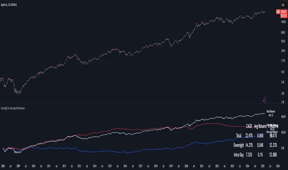
Overnight vs Intra-day Performance█ STRATEGY OVERVIEW
The "Overnight vs Intra-day Performance" indicator quantifies price behaviour differences between trading hours and overnight periods. It calculates cumulative returns, compound growth rates, and visualizes performance components across user-defined time windows. Designed for analytical use, it helps identify whether returns are primarily generated during market hours or overnight sessions.
█ USAGE
Use this indicator on Stocks and ETFs to visualise and compare intra-day vs overnight performance
█ KEY FEATURES
Return Segmentation : Separates total returns into overnight (close-to-open) and intraday (open-to-close) components
Growth Tracking : Shows simple cumulative returns and compound annual growth rates (CAGR)
█ VISUALIZATION SYSTEM
1. Time-Series
Overnight Returns (Red)
Intraday Returns (Blue)
Total Returns (White)
2. Summary Table
Displays CAGR
3. Price Chart Labels
Floating annotations showing absolute returns and CAGR
Color-coded to match plot series
█ PURPOSE
Quantify market behaviour disparities between active trading sessions and overnight positioning
Provide institutional-grade attribution analysis for returns generation
Enable tactical adjustment of trading schedules based on historical performance patterns
Serve as foundational research for session-specific trading strategies
█ IDEAL USERS
1. Portfolio Managers
Analyse overnight risk exposure across holdings
Optimize execution timing based on return distributions
2. Quantitative Researchers
Study market microstructure through time-segmented returns
Develop alpha models leveraging session-specific anomalies
3. Market Microstructure Analysts
Identify liquidity patterns in overnight vs daytime sessions
Research ETF premium/discount mechanics
4. Day Traders
Align trading hours with highest probability return windows
Avoid overnight gaps through informed position sizing
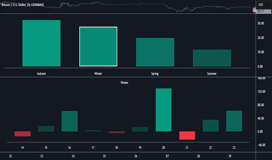
Market Performance by Yearly Seasons [LuxAlgo]The Market Performance by Yearly Seasons tool allows traders to analyze the average returns of the four seasons of the year and the raw returns of each separate season.
🔶 USAGE
By default, the tool displays the average returns for each season over the last 10 years in the form of bars, with the current session highlighted as a bordered bar.
Traders can choose to display the raw returns by year for each season separately and select the maximum number of seasons (years) to display.
🔹 Hemispheres
Traders can select the hemisphere in which they prefer to view the data.
🔹 Season Types
Traders can select the type of seasons between meteorological (by default) and astronomical.
The meteorological seasons are as follows:
Autumn: months from September to November
Winter: months from December to February
Spring: months from March to May
Summer: months from June to August
The astronomical seasons are as follows:
Autumn: from the equinox on September 22
Winter: from the solstice on December 21
Spring: from the equinox on March 20
Summer: from the solstice on June 21
🔹 Displaying the data
Traders can choose between two display modes, average returns by season or raw returns by season and year.
🔶 SETTINGS
Max seasons: Maximum number of seasons
Hemisphere: Select NORTHERN or SOUTHERN hemisphere
Season Type: Select the type of season - ASTRONOMICAL or METEOROLOGICAL
Display: Select display mode, all four seasons, or any one of them
🔹 Style
Bar Size & Autofit: Select the size of the bars and enable/disable the autofit feature
Labels Size: Select the label size
Colors & Gradient: Select the default color for bullish and bearish returns and enable/disable the gradient feature
Simple Volatility MomentumOverview:
The Simple Volatility Momentum indicator calculates the mean and standard deviation of the changes of price (returns) using various types of moving averages (Incremental, Rolling, and Exponential). With quantifying the dispersion of price data around the mean, statistical insights are provided on the volatility and the movements of price and returns. The indicator also ranks the mean absolute value of the changes of price over a specified time period which helps you assess the strength of the "trend" and "momentum" regardless of the direction of returns.
Simple Volatility Momentum
This indicator can be used for mean reversion strategies and "momentum" or trend based strategies.
The indicator calculates the average return as the momentum metric and then gets the moving average of the average return and standard deviations from average return average. On the options you can determine if you want to use 1 or 2 standard deviation bands or have both of them enabled.
Settings:
Source: By default it's at close.
M Length: This is the length of the "momentum".
Rank Length: This is the length of the rank calculation of absolute value of the average return
MA Type: This is the different type of calculations for the mean and standard deviation. By default its at incremental.
Smoothing factor: (Only used if you choose the exponential MA type.)
The absolute value of the average return helps you see the strength of the "momentum" and trend. If there is a low ranking of the absolute value of the average return then you can eventually expect it to increase which means that the average return is trending, leading to trending price moves. If the Mean ABS rank value is at or near the maximum value 100 and the average return is at -2 standard deviation from the mean, you can see it as the negative momentum or trend being "finished". Similarly, if the Mean ABS value is near or at the maximum value 100 and the average return is at +2 standard deviation from the mean, you can view the uptrend, as "finished" and the Mean ABS rank can't really go higher than 100.
Moving Average Calculations type:
Incremental: Incremental moving averages use an incremental approach to update the moving average by adding the newest data point and subtracting the oldest one.
Exponential: The exponential moving average gives more weight to recent data points while still considering older ones. This is achieved by applying a smooth factor to the previous EMA value and the current data point. EMA's react more quickly to recent changes in the data compared to simple moving averages, making them useful for short term trends and momentum in financial markets.
Rolling: The moving average is calculated by taking the average of a fixed number of data points within a defined window. As new data becomes available, the window moves forward and the average is recalculated. Rolling Moving Averages are useful for smoothing out short-fluctuations and identifying trends over time.
Important thing to note about indicators involving bands and "momentum" or "trend" or prices:
For the explanation we will assume that stock returns follow a normal distribution and price follows a log normal distribution. Please note that in the live market this assumption isn't always true. Many people incorrectly use standard deviations on prices and trade them as mean reversion strategies or overbought or oversold levels which is not what standard deviations are meant for. Assuming you have applied the log transformation on the standard deviation bands (if your input is raw price then you should use a log transformation to remove the skewness of price), and you have a range of 2 standard deviations from the mean, under the empirical rule with enough occurrences 95% of the values will be within the 2 standard deviation range. This doesn't mean that if price falls to the bottom of the 2 standard deviation bound, there is a 95% chance it will revert back to mean, this is incorrect and not how standard deviations or mean reversion works.
"MOMENTUM"
In finance "momentum" refers to the rate of change of a time series data point. It shows the persistence or tendency for a data series to continue moving in its current direction. In finance, "momentum" based strategies capitalize on the observed tendency of assets that have performed well (or poorly) in the recent past to continue performing well (or poorly) in the near future. This persistence is often observed in various financial instruments including stocks, currencies and commodities.
"Momentum" is commonly calculated with the average return, and relies on the assumption that assets with positive "momentum" or a positive average return will likely continue to perform well in the short to medium term, while assets with a negative average return are expected to continue underperforming. This average return or expected value is derived from historical observations and statistical analysis of previous price movements. However, real markets are subject to levels of efficiencies, market fluctuations, randomness, and may not always produce consistent returns over time involving momentum based strategies.
Mean Reversion:
In finance, the average return is an important parameter in mean reversion strategies. Using statistical methodologies, mean reversion strategies aim to exploit the deviations from the historical average return by identifying instances where current prices and their changes diverge from their expected levels based on past performance. This approach involves statistical analysis and predictive modelling techniques to check where and when the average rate of change is likely to revert towards the mean. It's important to know that mean reversion is a temporary state and will not always be present in a specific timeseries.
Using the average return over price offers several advantages in finance and trading since it is less sensitive to extreme price movements or outliers compared to raw price data. Price itself contains a distribution that is usually positively-skewed and has no upper bound. Mean reversion typically occurs in distributions where extreme values are followed by a tendency for the variable to return towards its mean over time, however the probability distribution of price has no tendency for values to revert towards any specific level. Instead, values may continue to increase without a bound. Returns themself contain more stationary behavior than price levels. Mean reversion strategies rely on the assumption that deviations from the mean will eventually revert back to the mean. Returns, being more likely to exhibit stationary, are better suited for mean reversion based strategies.
The distribution of returns are often more symmetrically distributed around their mean compared to price distributions. This symmetry makes it easier to identify deviations from the mean and assess the likelihood of mean reversion occurrence. Returns are also less sensitive to trends and long-term price movements compared to price levels. Mean reversion strategies aim to exploit deviations from mean, which can be obscured when analyzing raw price data since raw price is almost always trending. Returns can filter out the trend component of price movements, making it easier to identify opportunities.
Stationary Process: Implication that properties like mean and variance remain relatively constant over time.

MeanReversion - LogReturn/Vola ZScoreShows the z-Score of log-return (blue line) and volatility (black line). In statistics, the z-score is the number of standard deviations by which a value of a raw score is above or below the mean value.
This indicator aggregates z-score based on two indicators:
MeanReversion by Logarithmic Returns
MeanReversion by Volatility
Change the time period in bars for longer or shorter time frames. At a daily chart 252 mean on trading year, 21 mean one trading month.

Returns Model by TenozenHey there! I've been diving into the book "Paul Wilmott on Quantitative Finance," and I stumbled upon this cool model for calculating and modeling returns. Basically, it helps us figure out how much a price has changed over a set number of periods—I like to use 20 periods as a default. Once we get that rate of change value, we crunch some numbers to find the standard deviation and mean using all the historical data we have. That's the foundation of this model.
Now, let's talk about how to use it. This model shows us how returns and price behavior are connected. When returns hang out in the +1 to +2 standard deviation range, it usually means returns are about to drop, and vice versa. Often, this leads to corresponding price moves. But here's the thing: sometimes prices don't do what we expect. Why? It's because there's another hidden factor at play—I like to call it "power."
This "power" isn't something we can see directly, but it's there. Basically, when returns are within that standard deviation range, the market faces resistance when trying to move in its preferred direction, whether bullish or bearish. The strength of this "power" determines if the market will snap back to the average or go for a wild ride. It can show up as small price wiggles, big price jumps, or lightning-fast moves. By understanding this "power," we can get a better handle on what the market might do next and avoid getting blindsided. In the meantime, I couldn't explain "power" yet, but In the future, when I've learned enough, I'd love to share the model with you guys!
So... I'm planning to explore and share more models from this book as I learn, even if those pesky math formulas can be tough to crack. I hope you find this indicator as helpful as I do, and if you've got any suggestions or feedback, please feel free to share! Ciao!

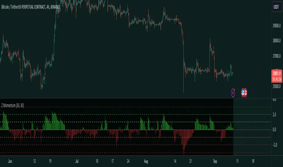
Z MomentumOverview
This is a Z-Scored Momentum Indicator. It allows you to understand the volatility of a financial instrument. This indicator calculates and displays the momentum of z-score returns expected value which can be used for finding the regime or for trading inefficiencies.
Indicator Purpose:
The primary purpose of the "Z-Score Momentum" indicator is to help traders identify potential trading opportunities by assessing how far the current returns of a financial instrument deviate from their historical mean returns. This analysis can aid in recognizing overbought or oversold conditions, trend strength, and potential reversal points.
Things to note:
A Z-Score is a measure of how many standard deviations a data point is away from the mean.
EV: Expected Value, which is basically the average outcome.
When the Z-Score Momentum is above 0, there is a positive Z-Score which indicates that the current returns of the financial instrument are above their historical mean returns over the specified return lookback period, which could mean Positive, Momentum, and in a extremely high Z-Score value, like above +2 Standard deviations it could indicate extreme conditions, but keep in mind this doesn't mean price will go down, this is just the EV.
When the Z-Score Momentum is below 0, there is negative Z-Score which indicates that the current returns of the financial instrument are below their historical mean returns which means you could expect negative returns. In extreme Z-Score situations like -2 Standard deviations this could indicate extreme conditions and the negative momentum is coming to an end.
TDLR:
Interpretation:
Positive Z-Score: When the Z-score is positive and increasing, it suggests that current returns are above their historical mean, indicating potential positive momentum.
Negative Z-Score: Conversely, a negative and decreasing Z-score implies that current returns are below their historical mean, suggesting potential negative momentum.
Extremely High or Low Z-Score: Extremely high (above +2) or low (below -2) Z-scores may indicate extreme market conditions that could be followed by reversals or significant price movements.
The lines on the Indicator highlight the Standard deviations of the Z-Score. It shows the Standard deviations 1,2,3 and -1,-2,-3.
Alpha Trading - Pseudo Laplace Z ScoreAlpha Trading - Pseudo Laplace Z Score
Slowly, very slowly a lot of quant and statistical methods have diffused the world of traditional technical analysis with the world of real math - VEPS (Volatility, Entropy, Probability and Statistics).
‘Alpha Trading' is showing the world how VEPS can show the best probabilities of success with your trading journey.
We send a big thank you to tradingview platform and pine coding team, for this great platform and the possibility to show the methods to trade with quant and statistical methods.
There appears to be resistance in the industry about these methods, so it is even more important now than ever, to support this awesome platform and amazing talented team at trading view and pine coders who enable us all with this wonderful platform to produce tools based on VEPS (Volatility, Entropy, Probability and Statistics).
The newest indicator from the Alpha Trading stable is the “Pseudo Laplace Z Score” which combines the established statistical method of z score applied on asset data. Which is based on our previous indicator called the “Alpha Trading – RMS-Z score”. We have made some optimizations, to give an even better fit to the specific returns of price. Optimizations are on the observation that returns are more Laplace distributed than Normal distributed.
figure 1: pink distribution of the real signal (BTC, 2D), gray is perfect theoretical Laplace distribution.
Therefore, the data is not Normal distributed, but Laplace distributed. Our new indicator calculates the real Z-Score of an underlying asset.
As Z Score is a standardized Normal distribution, it relies upon the definition of Normal distribution. If it deviates from this, it still can give useful information, but the absolute value (distance from the mean in standard deviations) is not reliable, and therefore the use of Normal distribution has some uncertainties.
Therefore, this indicator calculates a pseudo standard deviation, based on the Laplace distribution formulas and the relating Z Score.
By looking at the resulting distribution of the indicator itself, it is close to a perfect theoretical Normal distribution. It is much closer to the theoretical curve (gray), and thus indicates that the use of this approach is correct. Now we can show absolute values (i.e. distance to mean, in standard deviations) which can thus be considered to assist in determining the probabilities with your trading.
figure 2: distribution of indicator AT - Pseudo Laplace Z Score vs a theoretical perfect Normal distribution on BTC 4h
Looking at the indicator directly, it appears that the probability of 99% is crossed very rarely, like expected. Because only 1% of all candles we would expect this probability line to be exceeded.
figure 3: BTC 8h with AT-Pseudo Laplace Z Score
Coming back to the method of a Z Score in general. What is a Z-Score?
A Z-score is a numerical measurement that describes a value's relationship to the mean of a group of values. Z-score is measured in terms of standard deviations from the mean. If a Z-score is 0, it indicates that the data point's score is identical to the mean score. A Z-score of 1.0 would indicate a value that is one standard deviation from the mean. Z-scores may be positive or negative, with a positive value indicating the score is above the mean and a negative score indicating it is below the mean.
Simply put, a z-score (also called a standard score) gives you an idea of how far from the mean a data point is.
Basic guidelines How to Use this indicator:
Consider Entering a Long Position when the indicator is low. Best moves are generally when the indicator Turns yellow(outlier)
Consider Entering a Short Position when the indicator is high. Best moves are generally when the indicator Turns yellow(outlier)
Consider the 3 confidence interval lines (gray lines) at 90%, 95%, and 99%, as possible reversal point (with related probability that it is not getting exceeded 🡪 reversal)
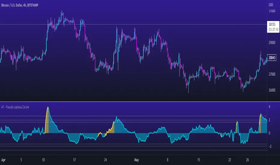
YoY or MoM ReturnsThis script is a technical indicator that calculates the year-over-year (YoY) or month-over-month (MoM) returns of a security.
The returns are then plotted on a chart, with positive returns colored in green and negative returns colored in red.

Monthly ReturnsDisplays monthly and yearly returns in tabular format along with maximum, minimum, average returns and standard deviations.
This uses boxes to build the table and as maximum boxes that could be used is 500, it displays up to 32 years of returns. However, for maximum, minimum, average and standard deviation calculations, it uses data from all months since inception.
This requires timeframe to be set to one month (1M). Cell widths correspond to years. For the first year, cell widths may be shorter and there could be overlap of numbers as nothing could be drawn before the first bar.
Provide sufficient space for the table to render properly. Zooming out or less space may lead to overlapping of numbers.

Performance Tablethis scrip is modified of Performance Table () of TradingView user @BeeHolder = Thank u very much.
-
@BeeHolder formula is based on daily basis,
but my calculation is based on respective day, week and month.
-
The formula of the calculation is (Current Close - Previous Close) * 100 / Previous Close, where Past value is:
1D = close 1 day before
5D = close 5 day before
1W - close 1 week before
4W = close 4 week before
1M - close 1 month before
3M - close 3 month before
6M - close 6 month before
12M - close 12 month before
52W - close 52 week before
Also table position cane be set.
thank you all
-

Annual Returns % Comparison [By MUQWISHI]Overview
The Annual Returns % Comparison indicator aimed to compare the historical annual percentage change of any two symbols. The indicator output shows a column-plot that was developed by two using a pine script table, so each period has pair columns showing the yearly percentage change for entered symbols.
Features
- Enter date range.
- Fill up with any two symbols.
- Choose the output data whether adjusted or not.
- Change the location of the table plot
- Color columns by a symbol.
- Size the height and width of columns.
- Color background, border, and text.
- The tooltip of the column value appears once the cursor sets above the specific column. As it seen below.
Let me know if you have any questions.
Thanks.
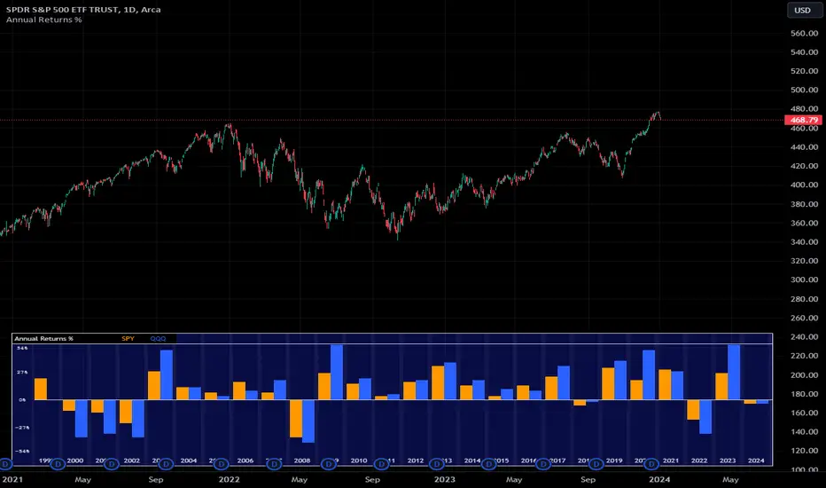
ln(close/20 sma) adjusted for time (BTC)(This indicator was designed for the BTC index chart)
Designed for Bitcoin. Plots the log of the close/20W SMA with a linear offset m*t, where m is the gradient I've chosen and t is the candle index. Anything above 1 is a mania phase/market cycle top. If it peaks around 0.92 and rolls over, it could be a local/market cycle top.
This will obviously not work at all in the long term as Bitcoin will not continue following the trend line on the log plot (you can even see it start to deviate in the Jan-Feb 2021 peaks where the indicator went to 1.15).
It identifies the 2011, 2013 (both of them), 2017 tops as being just above 1. It also identifies the 2019 local peak and 2021 market cycle top at ~0.94.
Feel free to change the gradient or even add a function to curve the straight line eventually. I made this for fun, feel free to use it as you wish.

Yearly Percentage ReturnsAn indicator that lets you visualize the historical Yearly Percentage returns of any symbol .
Key Features:
Displays the yearly returns from start to end of each year
Displays a table showing all yearly returns for current symbol
Displays start of each year as a vertical line
Displays up to 5 custom horizontal levels
Table Settings:
Enable table - Show/Hide the table
Size - Sets the size of the table
Position - Sets the position of the table on the screen
Direction - Sets the direction of the table to display the data (Vertically or Horizontally)