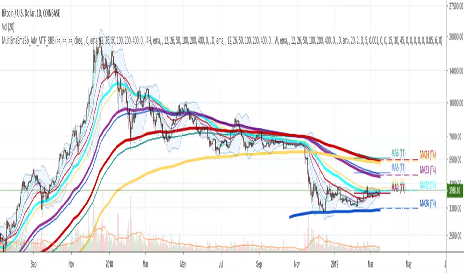
Multi SMA EMA WMA HMA BB (5x8 MAs Bollinger Bands) MAX MTF - RRBMulti SMA EMA WMA HMA 4x7 Moving Averages with Bollinger Bands MAX MTF by RagingRocketBull 2019
Version 1.0
All available MAX MTF versions are listed below (They are very similar and I don't want to publish them as separate indicators):
ver 1.0: 4x7 = 28 MTF MAs + 28 Levels + 3 BB = 59 < 64
ver 2.0: 5x6 = 30 MTF MAs + 30 Levels + 3 BB = 63 < 64
ver 3.0: 3x10 = 30 MTF MAs + 30 Levels + 3 BB = 63 < 64
ver 4.0: 5(4+1)x8 = 8 CurTF MAs + 32 MTF MAs + 20 Levels + 3 BB = 63 < 64
ver 5.0: 6(5+1)x6 = 6 CurTF MAs + 30 MTF MAs + 24 Levels + 3 BB = 63 < 64
ver 6.0: 4(3+1)x10 = 10 CurTF MAs + 30 MTF MAs + 20 Levels + 3 BB = 63 < 64
Fib numbers: 8, 13, 21, 34, 55, 89, 144, 233, 377
This indicator shows multiple MAs of any type SMA EMA WMA HMA etc with BB and MTF support, can show MAs as dynamically moving levels.
There are 4 MA groups + 1 BB group, a total of 4 TFs * 7 MAs = 28 MAs. You can assign any type/timeframe combo to a group, for example:
- EMAs 9,12,26,50,100,200,400 x H1, H4, D1, W1 (4 TFs x 7 MAs x 1 type)
- EMAs 8,13,21,30,34,50,55,89,100,144,200,233,377,400 x M15, H1 (2 TFs x 14 MAs x 1 type)
- D1 EMAs and SMAs 8,13,21,30,34,50,55,89,100,144,200,233,377,400 (1 TF x 14 MAs x 2 types)
- H1 WMAs 13,21,34,55,89,144,233; H4 HMAs 9,12,26,50,100,200,400; D1 EMAs 12,26,89,144,169,233,377; W1 SMAs 9,12,26,50,100,200,400 (4 TFs x 7 MAs x 4 types)
- +1 extra MA type/timeframe for BB
There are several versions: Simple, MTF, Pro MTF, Advanced MTF, MAX MTF and Ultimate MTF. This is the MAX MTF version. The Differences are listed below. All versions have BB
- Simple: you have 2 groups of MAs that can be assigned any type (5+5)
- MTF: +2 custom Timeframes for each group (2x5 MTF) +1 TF for BB, TF XY smoothing
- Pro MTF: 4 custom Timeframes for each group (4x3 MTF), 1 TF for BB, MA levels and show max bars back options
- Advanced MTF: +4 extra MAs/group (4x7 MTF), custom Ticker/Symbols, Timeframe <>= filter, Remove Duplicates Option
- MAX MTF: +2 subtypes/group, packed to the limit with max possible MAs/TFs: 4x7, 5x6, 3x10, 4(3+1)x10, 5(4+1)x8, 6(5+1)x6
- Ultimate MTF: +individual settings for each MA, custom Ticker/Symbols
MAX MTF version tests the limits of Pinescript trying to squeeze as many MAs/TFs as possible into a single indicator.
It's basically a maxed out Advanced version with subtypes allowing for mixed types within a group (i.e. both emas and smas in a single group/TF)
Pinescript has the following limits:
- max 40 security calls (6 calls are reserved for dupe checks and smoothing, 2 are used for BB, so only 32 calls are available)
- max 64 plot outputs (BB uses 3 outputs, so only 61 plot outputs are available)
- max 50000 (50kb) size of the compiled code
Based on those limits, you can only have the following MAs/TFs combos in a single script:
1. 4x7, 5x6, 3x10 - total number of MTF MAs must always be <= 32, and you can still have BB and Num Levels = total MAs, without any compromises
2. 5(4+1)x8, 6(5+1)x6, 4(3+1)x10 - you can use the Current Symbol/Timeframe as an extra (+1) fixed TF with the same number of MTF MAs
- you don't need to call security to display MAs on the Current Symbol/Timeframe, so the total number of MTF MAs remains the same and is still <= 32
- to fit that many MAs into the max 64 plot outputs limit you need to reduce the number of levels (not every MA Group will have corresponding levels)
Features:
- 4x7 = 28 MAs of any type
- 4x MTF groups with XY step line smoothing
- +1 extra TF/type for BB MAs
- 2 MA subtypes within each group/TF
- 4x7 = 28 MA levels with adjustable group offsets, indents and shift
- supports any existing type of MA: SMA, EMA, WMA, Hull Moving Average (HMA)
- custom tickers/symbols for each group
- show max bars back option
- show/hide both groups of MAs/levels/BB and individual MAs
- timeframe filter: show only MAs/Levels with TFs <>= Current TF
- hide MAs/Levels with duplicate TFs
- support for custom TFs that are not available in free accounts: 2D, 3D etc
- support for timeframes in H: H, 2H, 4H etc
Notes:
- Uses timeframe textbox instead of input resolution dropdown to allow for 240 120 and other custom TFs
- Uses symbol textbox instead of input symbol to avoid establishing multiple dummy security connections to the current ticker - otherwise empty symbols will prevent script from running
- Possible reasons for missing MAs on a chart:
- there may not be enough bars in history to start plotting it. For example, W1 EMA200 needs at least 200 bars on a weekly chart.
- for charts with low/fractional prices i.e. 0.00002 << 0.001 (default Y smoothing step) decrease Y smoothing as needed (set Y = 0.0000001) or disable it completely (set X,Y to 0,0)
- for charts with high price values i.e. 20000 >> 0.001 increase Y smoothing as needed (set Y = 10-20). Higher values exceeding MAs point density will cause it to disappear as there will be no points to plot. Different TFs may require diff adjustments
- TradingView Replay Mode UI and Pinescript security calls are limited to TFs >= D (D,2D,W,MN...) for free accounts
- attempting to plot any TF < D1 in Replay Mode will only result in straight lines, but all TFs will work properly in history and real-time modes. This is not a bug.
- Max Bars Back (num_bars) is limited to 5000 for free accounts (10000 for paid), will show error when exceeded. To plot on all available history set to 0 (default)
- Slow load/redraw times. This indicator becomes slower, its UI less responsive when:
- Pinescript Node.js graphics library is too slow and inefficient at plotting bars/objects in a browser window. Code optimization doesn't help much - the graphics engine is the main reason for general slowness.
- the chart has a long history (10000+ bars) in a browser's cache (you have scrolled back a couple of screens in a max zoom mode).
- Reload the page/Load a fresh chart and then apply the indicator or
- Switch to another Timeframe (old TF history will still remain in cache and that TF will be slow)
- in max possible zoom mode around 4500 bars can fit on 1 screen - this also slows down responsiveness. Reset Zoom level
- initial load and redraw times after a param change in UI also depend on TF. For example: D1/W1 - 2 sec, H1/H4 - 5-6 sec, M30 - 10 sec, M15/M5 - 4 sec, M1 - 5 sec. M30 usually has the longest history (up to 16000 bars) and W1 - the shortest (1000 bars).
- when indicator uses more MAs (plots) and timeframes it will redraw slower. Seems that up to 5 Timeframes is acceptable, but 6+ Timeframes can become very slow.
- show_last=last_bars plot limit doesn't affect load/redraw times, so it was removed from MA plot
- Max Bars Back (num_bars) default/custom set UI value doesn't seem to affect load/redraw times
- In max zoom mode all dynamic levels disappear (they behave like text)
- Dupe check includes symbol: symbol, tf, both subtypes - all must match for a duplicate group
- For the dupe check to work correctly a custom symbol must always include an exchange prefix. BB is not checked for dupes
Good Luck! Feel free to learn from/reuse the code to build your own indicators.
Recherche dans les scripts pour "12月4号是什么星座"

Multi SMA EMA WMA HMA BB (4x5 MAs Bollinger Bands) Adv MTF - RRBMulti SMA EMA WMA HMA 4x5 Moving Averages with Bollinger Bands Advanced MTF by RagingRocketBull 2019
Version 1.0
This indicator shows multiple MAs of any type SMA EMA WMA HMA etc with BB and MTF support, can show MAs as dynamically moving levels.
There are 4 MA groups + 1 BB group, a total of 4 TFs * 5 MAs = 20 MAs. You can assign any type/timeframe combo to a group, for example:
- EMAs 12,26,50,100,200 x H1, H4, D1, W1 (4 TFs x 5 MAs x 1 type)
- EMAs 8,10,13,21,30,50,55,100,200,400 x M15, H1 (2 TFs x 10 MAs x 1 type)
- D1 EMAs and SMAs 8,10,12,26,30,50,55,100,200,400 (1 TF x 10 MAs x 2 types)
- H1 WMAs 7,77,89,167,231; H4 HMAs 12,26,50,100,200; D1 EMAs 89,144,169,233,377; W1 SMAs 12,26,50,100,200 (4 TFs x 5 MAs x 4 types)
- +1 extra MA type/timeframe for BB
There are several versions: Simple, MTF, Pro MTF, Advanced MTF and Ultimate MTF. This is the Advanced MTF version. The Differences are listed below. All versions have BB
- Simple: you have 2 groups of MAs that can be assigned any type (5+5)
- MTF: +2 custom Timeframes for each group (2x5 MTF) +1 TF for BB, TF XY smoothing
- Pro MTF: 4 custom Timeframes for each group (4x3 MTF), 1 TF for BB, MA levels and show max bars back options
- Advanced MTF: +2 extra MAs/group (4x5 MTF), custom Ticker/Symbols, Timeframe <>= filter, Remove Duplicates Option
- Ultimate MTF: +individual settings for each MA, custom Ticker/Symbols
Features:
- 4x5 = 20 MAs of any type
- 4x MTF groups with XY step line smoothing
- +1 extra TF/type for BB MAs
- 4x5 = 20 MA levels with adjustable group offsets, indents and shift
- supports any existing type of MA: SMA, EMA, WMA, Hull Moving Average (HMA)
- custom tickers/symbols for each group - you can compare MAs of the same symbol across exchanges
- show max bars back option
- show/hide both groups of MAs/levels/BB and individual MAs
- timeframe filter: show only MAs/Levels with TFs <>= Current TF
- hide MAs/Levels with duplicate TFs
- support for custom TFs that are not available in free accounts: 2D, 3D etc
- support for timeframes in H: H, 2H, 4H etc
Notes:
- Uses timeframe textbox instead of input resolution dropdown to allow for 240 120 and other custom TFs
- Uses symbol textbox instead of input symbol to avoid establishing multiple dummy security connections to the current ticker - otherwise empty symbols will prevent script from running
- Possible reasons for missing MAs on a chart:
- there may not be enough bars in history to start plotting it. For example, W1 EMA200 needs at least 200 bars on a weekly chart.
- price << default Y smoothing step 5. For charts with low/fractional prices (i.e. 0.00002 << 5) adjust X Y smoothing as needed (set Y = 0.0000001) or disable it completely (set X,Y to 0,0)
- TradingView Replay Mode UI and Pinescript security calls are limited to TFs >= D (D,2D,W,MN...) for free accounts
- attempting to plot any TF < D1 in Replay Mode will only result in straight lines, but all TFs will work properly in history and real-time modes. This is not a bug.
- Max Bars Back (num_bars) is limited to 5000 for free accounts (10000 for paid), will show error when exceeded. To plot on all available history set to 0 (default)
- Slow load/redraw times. This indicator becomes slower, its UI less responsive when:
- Pinescript Node.js graphics library is too slow and inefficient at plotting bars/objects in a browser window. Code optimization doesn't help much - the graphics engine is the main reason for general slowness.
- the chart has a long history (10000+ bars) in a browser's cache (you have scrolled back a couple of screens in a max zoom mode).
- Reload the page/Load a fresh chart and then apply the indicator or
- Switch to another Timeframe (old TF history will still remain in cache and that TF will be slow)
- in max possible zoom mode around 4500 bars can fit on 1 screen - this also slows down responsiveness. Reset Zoom level
- initial load and redraw times after a param change in UI also depend on TF. For example:
D1/W1 - 2 sec, H1/H4 - 5-6 sec, M30 - 10 sec, M15/M5 - 4 sec, M1 - 5 sec.
M30 usually has the longest history (up to 16000 bars) and W1 - the shortest (1000 bars).
- when indicator uses more MAs (plots) and timeframes it will redraw slower. Seems that up to 5 Timeframes is acceptable, but 6+ Timeframes can become very slow.
- show_last=last_bars plot limit doesn't affect load/redraw times, so it was removed from MA plot
- Max Bars Back (num_bars) default/custom set UI value doesn't seem to affect load/redraw times
- In max zoom mode all dynamic levels disappear (they behave like text)
1. based on 3EmaBB, uses plot*, barssince and security functions
2. you can't set certain constants from input due to Pinescript limitations - change the code as needed, recompile and use as a private version
3. Levels = trackprice implementation
4. Show Max Bars Back = show_last implementation
5. swma has a fixed length = 4, alma and linreg have additional offset and smoothing params
6. Smoothing is applied by default for visual aesthetics on MTF. To use exact ma mtf values (lines with stair stepping) - disable it
Good Luck! You can explore, modify/reuse the code to build your own indicators.
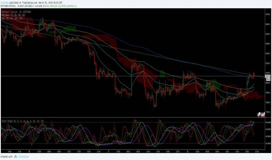
ShiftPower StochasticThis indicator is a combination of the following three slow stochastics commonly used.
ⓐ 5 - 3 - 3
ⓑ 10 - 6 - 6
ⓒ 20 - 12 - 12
( n - %k - %d )
I hope it helps. Thanks.
<한국어>
일반적으로 많이 사용하는 다음 3개의 슬로우 스토케스틱을 하나로 합친 지표입니다.
ⓐ 5 - 3 - 3
ⓑ 10 - 6 - 6
ⓒ 20 - 12 - 12
( n - %k - %d )
도움이 됐으면 좋겠습니다. 감사합니다.
MACD Crossover Backtest MACD – Moving Average Convergence Divergence. The MACD is calculated
by subtracting a 26-day moving average of a security's price from a
12-day moving average of its price. The result is an indicator that
oscillates above and below zero. When the MACD is above zero, it means
the 12-day moving average is higher than the 26-day moving average.
This is bullish as it shows that current expectations (i.e., the 12-day
moving average) are more bullish than previous expectations (i.e., the
26-day average). This implies a bullish, or upward, shift in the supply/demand
lines. When the MACD falls below zero, it means that the 12-day moving average
is less than the 26-day moving average, implying a bearish shift in the
supply/demand lines.
A 9-day moving average of the MACD (not of the security's price) is usually
plotted on top of the MACD indicator. This line is referred to as the "signal"
line. The signal line anticipates the convergence of the two moving averages
(i.e., the movement of the MACD toward the zero line).
Let's consider the rational behind this technique. The MACD is the difference
between two moving averages of price. When the shorter-term moving average rises
above the longer-term moving average (i.e., the MACD rises above zero), it means
that investor expectations are becoming more bullish (i.e., there has been an
upward shift in the supply/demand lines). By plotting a 9-day moving average of
the MACD, we can see the changing of expectations (i.e., the shifting of the
supply/demand lines) as they occur.
You can change long to short in the Input Settings
WARNING:
- For purpose educate only
- This script to change bars colors.

Forex session - Opening Range- Jayy fixed updatedOpening Range (OR) for Forex 24 hour regular session. This is not for regular market day sessions addressed in a separate script.
This script fixes four issues:
syntax error when code compiles
messed up opening range the day after a holiday Monday
flaky plotting of the opening range and targets that required page reloading
TradingView problems with starting forex session at 1700 hours EST/EDT when using certain securities eg FX_IDC currently (Jan 2017)
Additions in his code are more options for trading range
Time compensation option for some securities that incorrectly start sessions at 1200 hrs instead of 1700 hrs NY time
- this glitch is likely temporary but present when this script update was created
More opening range time period choices
Opening Range Targets:
Opening Range Targets as per Leaf_West
Targets are set at 127% , 162%, 200 %, 262 %, 362%, 423%, 685%, 1109% and 1794% and this can be traded intraday using methods described here charts-by-leaf.com I also have some Leaf West PDFs that describe how the targets are set and how they are traded. There are others that use opening range.
The Time Session Glitch and the Fix:
The script will correctly default to 1700 hrs to 1700hrs EDT/EST session for FXCM.
Strangely some securities appear to erroneously start their session at 1200 hrs ie. My guess is that they are somehow tied to GMT+0 instead of New York time (GMT+5). See this for yourself by selecting EURUSD using the FXCM exchange (FX:EURUSD) and then EURUSD from the IDC exchange (FX_IDC:EURUSD). The FX-IDC session opening range starts 5 hours
before it actually should at 1700 hrs EDT/EST. To correct for this I have implemented an automatic fix (default) and a user selected "5 hour time shift adjust. ment needed on some securities".
There is also a 4 hour time shift button which might be necessary when New York reverts from Eastern Standard Time
to Eastern Daylight Time (1 hour difference) in March (and then back again in November). In the default auto adjust mode you will need to select the 1 hour time shift. That is if this glitch still exists at that time.
I have looked at other scripts, other than my own and where the script is available, that need to use information about the opening bar and all have the same time shift issue
What are the choices for Opening Range?
The dialogue box offers the standard TradingView options.
Also where you see Pick Opening Range 1 to 12 hours , SET TO 0 To USE LINE ABOVE TO DETERMINE OR LENGTH
As the note says a number other than 0 will override the standard options from the line above
The dialogue box below in offers choices by hours 1 to 12. A number greater than 12 will still only give
720 minutes (12 hours) for the length of Opening Range.
What sessions within the FOREX time-frame are available?
The default is 1700 hours to 1700 hours EST/EDT
Check any one (only one) of the time periods to change the opening range period to suit.
New York opens at 8:00 am to 5:00 pm EST (EDT)
Tokyo opens at 7:00 pm to 4:00 am EST (EDT)
Sydney opens at 5:00 pm to 2:00 am EST (EDT)
London opens at 3:00 am to 12:00 noon EST (EDT)
There is a build your own session (click the button to select)
The two lines for inputting session times are almost identical except that the second line starts the be the same as each other.
The default for the build your own session is 2200 hours to 2200 hours. As of the time of publishing this plots EURUSD FX-IDC just right. The GMT+5 and GMT+4 do not apply to this selection.
See my comments above on this strange aberration.
The script originated from work done by Chris Moody. It has changed significantly but there are remnants of that script lurking within.
Script is free to all - that way you can see what is inside
Cheers Jayy

MACD Crossover MACD – Moving Average Convergence Divergence. The MACD is calculated
by subtracting a 26-day moving average of a security's price from a
12-day moving average of its price. The result is an indicator that
oscillates above and below zero. When the MACD is above zero, it means
the 12-day moving average is higher than the 26-day moving average.
This is bullish as it shows that current expectations (i.e., the 12-day
moving average) are more bullish than previous expectations (i.e., the
26-day average). This implies a bullish, or upward, shift in the supply/demand
lines. When the MACD falls below zero, it means that the 12-day moving average
is less than the 26-day moving average, implying a bearish shift in the
supply/demand lines.
A 9-day moving average of the MACD (not of the security's price) is usually
plotted on top of the MACD indicator. This line is referred to as the "signal"
line. The signal line anticipates the convergence of the two moving averages
(i.e., the movement of the MACD toward the zero line).
Let's consider the rational behind this technique. The MACD is the difference
between two moving averages of price. When the shorter-term moving average rises
above the longer-term moving average (i.e., the MACD rises above zero), it means
that investor expectations are becoming more bullish (i.e., there has been an
upward shift in the supply/demand lines). By plotting a 9-day moving average of
the MACD, we can see the changing of expectations (i.e., the shifting of the
supply/demand lines) as they occur.

Dynamic Equity Allocation Model//@version=6
indicator('Dynamic Equity Allocation Model', shorttitle = 'DEAM', overlay = false, precision = 1, scale = scale.right, max_bars_back = 500)
// DYNAMIC EQUITY ALLOCATION MODEL
// Quantitative framework for dynamic portfolio allocation between stocks and cash.
// Analyzes five dimensions: market regime, risk metrics, valuation, sentiment,
// and macro conditions to generate allocation recommendations (0-100% equity).
//
// Uses real-time data from TradingView including fundamentals (P/E, ROE, ERP),
// volatility indicators (VIX), credit spreads, yield curves, and market structure.
// INPUT PARAMETERS
group1 = 'Model Configuration'
model_type = input.string('Adaptive', 'Allocation Model Type', options = , group = group1, tooltip = 'Conservative: Slower to increase equity, Aggressive: Faster allocation changes, Adaptive: Dynamic based on regime')
use_crisis_detection = input.bool(true, 'Enable Crisis Detection System', group = group1, tooltip = 'Automatic detection and response to crisis conditions')
use_regime_model = input.bool(true, 'Use Market Regime Detection', group = group1, tooltip = 'Identify Bull/Bear/Crisis regimes for dynamic allocation')
group2 = 'Portfolio Risk Management'
target_portfolio_volatility = input.float(12.0, 'Target Portfolio Volatility (%)', minval = 3, maxval = 20, step = 0.5, group = group2, tooltip = 'Target portfolio volatility (Cash reduces volatility: 50% Equity = ~10% vol, 100% Equity = ~20% vol)')
max_portfolio_drawdown = input.float(15.0, 'Maximum Portfolio Drawdown (%)', minval = 5, maxval = 35, step = 2.5, group = group2, tooltip = 'Maximum acceptable PORTFOLIO drawdown (not market drawdown - portfolio with cash has lower drawdown)')
enable_portfolio_risk_scaling = input.bool(true, 'Enable Portfolio Risk Scaling', group = group2, tooltip = 'Scale allocation based on actual portfolio risk characteristics (recommended)')
risk_lookback = input.int(252, 'Risk Calculation Period (Days)', minval = 60, maxval = 504, group = group2, tooltip = 'Period for calculating volatility and risk metrics')
group3 = 'Component Weights (Total = 100%)'
w_regime = input.float(35.0, 'Market Regime Weight (%)', minval = 0, maxval = 100, step = 5, group = group3)
w_risk = input.float(25.0, 'Risk Metrics Weight (%)', minval = 0, maxval = 100, step = 5, group = group3)
w_valuation = input.float(20.0, 'Valuation Weight (%)', minval = 0, maxval = 100, step = 5, group = group3)
w_sentiment = input.float(15.0, 'Sentiment Weight (%)', minval = 0, maxval = 100, step = 5, group = group3)
w_macro = input.float(5.0, 'Macro Weight (%)', minval = 0, maxval = 100, step = 5, group = group3)
group4 = 'Crisis Detection Thresholds'
crisis_vix_threshold = input.float(40, 'Crisis VIX Level', minval = 30, maxval = 80, group = group4, tooltip = 'VIX level indicating crisis conditions (COVID peaked at 82)')
crisis_drawdown_threshold = input.float(15, 'Crisis Drawdown Threshold (%)', minval = 10, maxval = 30, group = group4, tooltip = 'Market drawdown indicating crisis conditions')
crisis_credit_spread = input.float(500, 'Crisis Credit Spread (bps)', minval = 300, maxval = 1000, group = group4, tooltip = 'High yield spread indicating crisis conditions')
group5 = 'Display Settings'
show_components = input.bool(false, 'Show Component Breakdown', group = group5, tooltip = 'Display individual component analysis lines')
show_regime_background = input.bool(true, 'Show Dynamic Background', group = group5, tooltip = 'Color background based on allocation signals')
show_reference_lines = input.bool(false, 'Show Reference Lines', group = group5, tooltip = 'Display allocation percentage reference lines')
show_dashboard = input.bool(true, 'Show Analytics Dashboard', group = group5, tooltip = 'Display comprehensive analytics table')
show_confidence_bands = input.bool(false, 'Show Confidence Bands', group = group5, tooltip = 'Display uncertainty quantification bands')
smoothing_period = input.int(3, 'Smoothing Period', minval = 1, maxval = 10, group = group5, tooltip = 'Smoothing to reduce allocation noise')
background_intensity = input.int(95, 'Background Intensity (%)', minval = 90, maxval = 99, group = group5, tooltip = 'Higher values = more transparent background')
// Styling Options
color_scheme = input.string('EdgeTools', 'Color Theme', options = , group = 'Appearance', tooltip = 'Professional color themes')
use_dark_mode = input.bool(true, 'Optimize for Dark Theme', group = 'Appearance')
main_line_width = input.int(3, 'Main Line Width', minval = 1, maxval = 5, group = 'Appearance')
// DATA RETRIEVAL
// Market Data
sp500 = request.security('SPY', timeframe.period, close)
sp500_high = request.security('SPY', timeframe.period, high)
sp500_low = request.security('SPY', timeframe.period, low)
sp500_volume = request.security('SPY', timeframe.period, volume)
// Volatility Indicators
vix = request.security('VIX', timeframe.period, close)
vix9d = request.security('VIX9D', timeframe.period, close)
vxn = request.security('VXN', timeframe.period, close)
// Fixed Income and Credit
us2y = request.security('US02Y', timeframe.period, close)
us10y = request.security('US10Y', timeframe.period, close)
us3m = request.security('US03MY', timeframe.period, close)
hyg = request.security('HYG', timeframe.period, close)
lqd = request.security('LQD', timeframe.period, close)
tlt = request.security('TLT', timeframe.period, close)
// Safe Haven Assets
gold = request.security('GLD', timeframe.period, close)
usd = request.security('DXY', timeframe.period, close)
yen = request.security('JPYUSD', timeframe.period, close)
// Financial data with fallback values
get_financial_data(symbol, fin_id, period, fallback) =>
data = request.financial(symbol, fin_id, period, ignore_invalid_symbol = true)
na(data) ? fallback : data
// SPY fundamental metrics
spy_earnings_per_share = get_financial_data('AMEX:SPY', 'EARNINGS_PER_SHARE_BASIC', 'TTM', 20.0)
spy_operating_earnings_yield = get_financial_data('AMEX:SPY', 'OPERATING_EARNINGS_YIELD', 'FY', 4.5)
spy_dividend_yield = get_financial_data('AMEX:SPY', 'DIVIDENDS_YIELD', 'FY', 1.8)
spy_buyback_yield = get_financial_data('AMEX:SPY', 'BUYBACK_YIELD', 'FY', 2.0)
spy_net_margin = get_financial_data('AMEX:SPY', 'NET_MARGIN', 'TTM', 12.0)
spy_debt_to_equity = get_financial_data('AMEX:SPY', 'DEBT_TO_EQUITY', 'FY', 0.5)
spy_return_on_equity = get_financial_data('AMEX:SPY', 'RETURN_ON_EQUITY', 'FY', 15.0)
spy_free_cash_flow = get_financial_data('AMEX:SPY', 'FREE_CASH_FLOW', 'TTM', 100000000)
spy_ebitda = get_financial_data('AMEX:SPY', 'EBITDA', 'TTM', 200000000)
spy_pe_forward = get_financial_data('AMEX:SPY', 'PRICE_EARNINGS_FORWARD', 'FY', 18.0)
spy_total_debt = get_financial_data('AMEX:SPY', 'TOTAL_DEBT', 'FY', 500000000)
spy_total_equity = get_financial_data('AMEX:SPY', 'TOTAL_EQUITY', 'FY', 1000000000)
spy_enterprise_value = get_financial_data('AMEX:SPY', 'ENTERPRISE_VALUE', 'FY', 30000000000)
spy_revenue_growth = get_financial_data('AMEX:SPY', 'REVENUE_ONE_YEAR_GROWTH', 'TTM', 5.0)
// Market Breadth Indicators
nya = request.security('NYA', timeframe.period, close)
rut = request.security('IWM', timeframe.period, close)
// Sector Performance
xlk = request.security('XLK', timeframe.period, close)
xlu = request.security('XLU', timeframe.period, close)
xlf = request.security('XLF', timeframe.period, close)
// MARKET REGIME DETECTION
// Calculate Market Trend
sma_20 = ta.sma(sp500, 20)
sma_50 = ta.sma(sp500, 50)
sma_200 = ta.sma(sp500, 200)
ema_10 = ta.ema(sp500, 10)
// Market Structure Score
trend_strength = 0.0
trend_strength := trend_strength + (sp500 > sma_20 ? 1 : -1)
trend_strength := trend_strength + (sp500 > sma_50 ? 1 : -1)
trend_strength := trend_strength + (sp500 > sma_200 ? 2 : -2)
trend_strength := trend_strength + (sma_50 > sma_200 ? 2 : -2)
// Volatility Regime
returns = math.log(sp500 / sp500 )
realized_vol_20d = ta.stdev(returns, 20) * math.sqrt(252) * 100
realized_vol_60d = ta.stdev(returns, 60) * math.sqrt(252) * 100
ewma_vol = ta.ema(math.pow(returns, 2), 20)
realized_vol = math.sqrt(ewma_vol * 252) * 100
vol_premium = vix - realized_vol
// Drawdown Calculation
running_max = ta.highest(sp500, risk_lookback)
current_drawdown = (running_max - sp500) / running_max * 100
// Regime Score
regime_score = 0.0
// Trend Component (40%)
if trend_strength >= 4
regime_score := regime_score + 40
regime_score
else if trend_strength >= 2
regime_score := regime_score + 30
regime_score
else if trend_strength >= 0
regime_score := regime_score + 20
regime_score
else if trend_strength >= -2
regime_score := regime_score + 10
regime_score
else
regime_score := regime_score + 0
regime_score
// Volatility Component (30%)
if vix < 15
regime_score := regime_score + 30
regime_score
else if vix < 20
regime_score := regime_score + 25
regime_score
else if vix < 25
regime_score := regime_score + 15
regime_score
else if vix < 35
regime_score := regime_score + 5
regime_score
else
regime_score := regime_score + 0
regime_score
// Drawdown Component (30%)
if current_drawdown < 3
regime_score := regime_score + 30
regime_score
else if current_drawdown < 7
regime_score := regime_score + 20
regime_score
else if current_drawdown < 12
regime_score := regime_score + 10
regime_score
else if current_drawdown < 20
regime_score := regime_score + 5
regime_score
else
regime_score := regime_score + 0
regime_score
// Classify Regime
market_regime = regime_score >= 80 ? 'Strong Bull' : regime_score >= 60 ? 'Bull Market' : regime_score >= 40 ? 'Neutral' : regime_score >= 20 ? 'Correction' : regime_score >= 10 ? 'Bear Market' : 'Crisis'
// RISK-BASED ALLOCATION
// Calculate Market Risk
parkinson_hl = math.log(sp500_high / sp500_low)
parkinson_vol = parkinson_hl / (2 * math.sqrt(math.log(2))) * math.sqrt(252) * 100
garman_klass_vol = math.sqrt((0.5 * math.pow(math.log(sp500_high / sp500_low), 2) - (2 * math.log(2) - 1) * math.pow(math.log(sp500 / sp500 ), 2)) * 252) * 100
market_volatility_20d = math.max(ta.stdev(returns, 20) * math.sqrt(252) * 100, parkinson_vol)
market_volatility_60d = ta.stdev(returns, 60) * math.sqrt(252) * 100
market_drawdown = current_drawdown
// Initialize risk allocation
risk_allocation = 50.0
if enable_portfolio_risk_scaling
// Volatility-based allocation
vol_based_allocation = target_portfolio_volatility / math.max(market_volatility_20d, 5.0) * 100
vol_based_allocation := math.max(0, math.min(100, vol_based_allocation))
// Drawdown-based allocation
dd_based_allocation = 100.0
if market_drawdown > 1.0
dd_based_allocation := max_portfolio_drawdown / market_drawdown * 100
dd_based_allocation := math.max(0, math.min(100, dd_based_allocation))
dd_based_allocation
// Combine (conservative)
risk_allocation := math.min(vol_based_allocation, dd_based_allocation)
// Dynamic adjustment
current_equity_estimate = 50.0
estimated_portfolio_vol = current_equity_estimate / 100 * market_volatility_20d
estimated_portfolio_dd = current_equity_estimate / 100 * market_drawdown
vol_utilization = estimated_portfolio_vol / target_portfolio_volatility
dd_utilization = estimated_portfolio_dd / max_portfolio_drawdown
risk_utilization = math.max(vol_utilization, dd_utilization)
risk_adjustment_factor = 1.0
if risk_utilization > 1.0
risk_adjustment_factor := math.exp(-0.5 * (risk_utilization - 1.0))
risk_adjustment_factor := math.max(0.5, risk_adjustment_factor)
risk_adjustment_factor
else if risk_utilization < 0.9
risk_adjustment_factor := 1.0 + 0.2 * math.log(1.0 / risk_utilization)
risk_adjustment_factor := math.min(1.3, risk_adjustment_factor)
risk_adjustment_factor
risk_allocation := risk_allocation * risk_adjustment_factor
risk_allocation
else
vol_scalar = target_portfolio_volatility / math.max(market_volatility_20d, 10)
vol_scalar := math.min(1.5, math.max(0.2, vol_scalar))
drawdown_penalty = 0.0
if current_drawdown > max_portfolio_drawdown
drawdown_penalty := (current_drawdown - max_portfolio_drawdown) / max_portfolio_drawdown
drawdown_penalty := math.min(1.0, drawdown_penalty)
drawdown_penalty
risk_allocation := 100 * vol_scalar * (1 - drawdown_penalty)
risk_allocation
risk_allocation := math.max(0, math.min(100, risk_allocation))
// VALUATION ANALYSIS
// Valuation Metrics
actual_pe_ratio = spy_earnings_per_share > 0 ? sp500 / spy_earnings_per_share : spy_pe_forward
actual_earnings_yield = nz(spy_operating_earnings_yield, 0) > 0 ? spy_operating_earnings_yield : 100 / actual_pe_ratio
total_shareholder_yield = spy_dividend_yield + spy_buyback_yield
// Equity Risk Premium (multi-method calculation)
method1_erp = actual_earnings_yield - us10y
method2_erp = actual_earnings_yield + spy_buyback_yield - us10y
payout_ratio = spy_dividend_yield > 0 and actual_earnings_yield > 0 ? spy_dividend_yield / actual_earnings_yield : 0.4
sustainable_growth = spy_return_on_equity * (1 - payout_ratio) / 100
method3_erp = spy_dividend_yield + sustainable_growth * 100 - us10y
implied_growth = spy_revenue_growth * 0.7
method4_erp = total_shareholder_yield + implied_growth - us10y
equity_risk_premium = method1_erp * 0.35 + method2_erp * 0.30 + method3_erp * 0.20 + method4_erp * 0.15
ev_ebitda_ratio = spy_enterprise_value > 0 and spy_ebitda > 0 ? spy_enterprise_value / spy_ebitda : 15.0
debt_equity_health = spy_debt_to_equity < 1.0 ? 1.2 : spy_debt_to_equity < 2.0 ? 1.0 : 0.8
// Valuation Score
base_valuation_score = 50.0
if equity_risk_premium > 4
base_valuation_score := 95
base_valuation_score
else if equity_risk_premium > 3
base_valuation_score := 85
base_valuation_score
else if equity_risk_premium > 2
base_valuation_score := 70
base_valuation_score
else if equity_risk_premium > 1
base_valuation_score := 55
base_valuation_score
else if equity_risk_premium > 0
base_valuation_score := 40
base_valuation_score
else if equity_risk_premium > -1
base_valuation_score := 25
base_valuation_score
else
base_valuation_score := 10
base_valuation_score
growth_adjustment = spy_revenue_growth > 10 ? 10 : spy_revenue_growth > 5 ? 5 : 0
margin_adjustment = spy_net_margin > 15 ? 5 : spy_net_margin < 8 ? -5 : 0
roe_adjustment = spy_return_on_equity > 20 ? 5 : spy_return_on_equity < 10 ? -5 : 0
valuation_score = base_valuation_score + growth_adjustment + margin_adjustment + roe_adjustment
valuation_score := math.max(0, math.min(100, valuation_score * debt_equity_health))
// SENTIMENT ANALYSIS
// VIX Term Structure
vix_term_structure = vix9d > 0 ? vix / vix9d : 1
backwardation = vix_term_structure > 1.05
steep_backwardation = vix_term_structure > 1.15
// Safe Haven Flows
gold_momentum = ta.roc(gold, 20)
dollar_momentum = ta.roc(usd, 20)
yen_momentum = ta.roc(yen, 20)
treasury_momentum = ta.roc(tlt, 20)
safe_haven_flow = gold_momentum * 0.3 + treasury_momentum * 0.3 + dollar_momentum * 0.25 + yen_momentum * 0.15
// Advanced Sentiment Analysis
vix_percentile = ta.percentrank(vix, 252)
vix_zscore = (vix - ta.sma(vix, 252)) / ta.stdev(vix, 252)
vix_momentum = ta.roc(vix, 5)
vvix_proxy = ta.stdev(vix_momentum, 20) * math.sqrt(252)
risk_reversal_proxy = (vix - realized_vol) / realized_vol
// Sentiment Score
base_sentiment = 50.0
vix_adjustment = 0.0
if vix_zscore < -1.5
vix_adjustment := 40
vix_adjustment
else if vix_zscore < -0.5
vix_adjustment := 20
vix_adjustment
else if vix_zscore < 0.5
vix_adjustment := 0
vix_adjustment
else if vix_zscore < 1.5
vix_adjustment := -20
vix_adjustment
else
vix_adjustment := -40
vix_adjustment
term_structure_adjustment = backwardation ? -15 : steep_backwardation ? -30 : 5
vvix_adjustment = vvix_proxy > 2.0 ? -10 : vvix_proxy < 1.0 ? 10 : 0
sentiment_score = base_sentiment + vix_adjustment + term_structure_adjustment + vvix_adjustment
sentiment_score := math.max(0, math.min(100, sentiment_score))
// MACRO ANALYSIS
// Yield Curve
yield_spread_2_10 = us10y - us2y
yield_spread_3m_10 = us10y - us3m
// Credit Conditions
hyg_return = ta.roc(hyg, 20)
lqd_return = ta.roc(lqd, 20)
tlt_return = ta.roc(tlt, 20)
hyg_duration = 4.0
lqd_duration = 8.0
tlt_duration = 17.0
hyg_log_returns = math.log(hyg / hyg )
lqd_log_returns = math.log(lqd / lqd )
hyg_volatility = ta.stdev(hyg_log_returns, 20) * math.sqrt(252)
lqd_volatility = ta.stdev(lqd_log_returns, 20) * math.sqrt(252)
hyg_yield_proxy = -math.log(hyg / hyg ) * 100
lqd_yield_proxy = -math.log(lqd / lqd ) * 100
tlt_yield = us10y
hyg_spread = (hyg_yield_proxy - tlt_yield) * 100
lqd_spread = (lqd_yield_proxy - tlt_yield) * 100
hyg_distance = (hyg - ta.lowest(hyg, 252)) / (ta.highest(hyg, 252) - ta.lowest(hyg, 252))
lqd_distance = (lqd - ta.lowest(lqd, 252)) / (ta.highest(lqd, 252) - ta.lowest(lqd, 252))
default_risk_proxy = 2.0 - (hyg_distance + lqd_distance)
credit_spread = hyg_spread * 0.5 + (hyg_volatility - lqd_volatility) * 1000 * 0.3 + default_risk_proxy * 200 * 0.2
credit_spread := math.max(50, credit_spread)
credit_market_health = hyg_return > lqd_return ? 1 : -1
flight_to_quality = tlt_return > (hyg_return + lqd_return) / 2
// Macro Score
macro_score = 50.0
yield_curve_score = 0
if yield_spread_2_10 > 1.5 and yield_spread_3m_10 > 2
yield_curve_score := 40
yield_curve_score
else if yield_spread_2_10 > 0.5 and yield_spread_3m_10 > 1
yield_curve_score := 30
yield_curve_score
else if yield_spread_2_10 > 0 and yield_spread_3m_10 > 0
yield_curve_score := 20
yield_curve_score
else if yield_spread_2_10 < 0 or yield_spread_3m_10 < 0
yield_curve_score := 10
yield_curve_score
else
yield_curve_score := 5
yield_curve_score
credit_conditions_score = 0
if credit_spread < 200 and not flight_to_quality
credit_conditions_score := 30
credit_conditions_score
else if credit_spread < 400 and credit_market_health > 0
credit_conditions_score := 20
credit_conditions_score
else if credit_spread < 600
credit_conditions_score := 15
credit_conditions_score
else if credit_spread < 1000
credit_conditions_score := 10
credit_conditions_score
else
credit_conditions_score := 0
credit_conditions_score
financial_stability_score = 0
if spy_debt_to_equity < 0.5 and spy_return_on_equity > 15
financial_stability_score := 20
financial_stability_score
else if spy_debt_to_equity < 1.0 and spy_return_on_equity > 10
financial_stability_score := 15
financial_stability_score
else if spy_debt_to_equity < 1.5
financial_stability_score := 10
financial_stability_score
else
financial_stability_score := 5
financial_stability_score
macro_score := yield_curve_score + credit_conditions_score + financial_stability_score
macro_score := math.max(0, math.min(100, macro_score))
// CRISIS DETECTION
crisis_indicators = 0
if vix > crisis_vix_threshold
crisis_indicators := crisis_indicators + 1
crisis_indicators
if vix > 60
crisis_indicators := crisis_indicators + 2
crisis_indicators
if current_drawdown > crisis_drawdown_threshold
crisis_indicators := crisis_indicators + 1
crisis_indicators
if current_drawdown > 25
crisis_indicators := crisis_indicators + 1
crisis_indicators
if credit_spread > crisis_credit_spread
crisis_indicators := crisis_indicators + 1
crisis_indicators
sp500_roc_5 = ta.roc(sp500, 5)
tlt_roc_5 = ta.roc(tlt, 5)
if sp500_roc_5 < -10 and tlt_roc_5 < -5
crisis_indicators := crisis_indicators + 2
crisis_indicators
volume_spike = sp500_volume > ta.sma(sp500_volume, 20) * 2
sp500_roc_1 = ta.roc(sp500, 1)
if volume_spike and sp500_roc_1 < -3
crisis_indicators := crisis_indicators + 1
crisis_indicators
is_crisis = crisis_indicators >= 3
is_severe_crisis = crisis_indicators >= 5
// FINAL ALLOCATION CALCULATION
// Convert regime to base allocation
regime_allocation = market_regime == 'Strong Bull' ? 100 : market_regime == 'Bull Market' ? 80 : market_regime == 'Neutral' ? 60 : market_regime == 'Correction' ? 40 : market_regime == 'Bear Market' ? 20 : 0
// Normalize weights
total_weight = w_regime + w_risk + w_valuation + w_sentiment + w_macro
w_regime_norm = w_regime / total_weight
w_risk_norm = w_risk / total_weight
w_valuation_norm = w_valuation / total_weight
w_sentiment_norm = w_sentiment / total_weight
w_macro_norm = w_macro / total_weight
// Calculate Weighted Allocation
weighted_allocation = regime_allocation * w_regime_norm + risk_allocation * w_risk_norm + valuation_score * w_valuation_norm + sentiment_score * w_sentiment_norm + macro_score * w_macro_norm
// Apply Crisis Override
if use_crisis_detection
if is_severe_crisis
weighted_allocation := math.min(weighted_allocation, 10)
weighted_allocation
else if is_crisis
weighted_allocation := math.min(weighted_allocation, 25)
weighted_allocation
// Model Type Adjustment
model_adjustment = 0.0
if model_type == 'Conservative'
model_adjustment := -10
model_adjustment
else if model_type == 'Aggressive'
model_adjustment := 10
model_adjustment
else if model_type == 'Adaptive'
recent_return = (sp500 - sp500 ) / sp500 * 100
if recent_return > 5
model_adjustment := 5
model_adjustment
else if recent_return < -5
model_adjustment := -5
model_adjustment
// Apply adjustment and bounds
final_allocation = weighted_allocation + model_adjustment
final_allocation := math.max(0, math.min(100, final_allocation))
// Smooth allocation
smoothed_allocation = ta.sma(final_allocation, smoothing_period)
// Calculate portfolio risk metrics (only for internal alerts)
actual_portfolio_volatility = smoothed_allocation / 100 * market_volatility_20d
actual_portfolio_drawdown = smoothed_allocation / 100 * current_drawdown
// VISUALIZATION
// Color definitions
var color primary_color = #2196F3
var color bullish_color = #4CAF50
var color bearish_color = #FF5252
var color neutral_color = #808080
var color text_color = color.white
var color bg_color = #000000
var color table_bg_color = #1E1E1E
var color header_bg_color = #2D2D2D
switch color_scheme // Apply color scheme
'Gold' =>
primary_color := use_dark_mode ? #FFD700 : #DAA520
bullish_color := use_dark_mode ? #FFA500 : #FF8C00
bearish_color := use_dark_mode ? #FF5252 : #D32F2F
neutral_color := use_dark_mode ? #C0C0C0 : #808080
text_color := use_dark_mode ? color.white : color.black
bg_color := use_dark_mode ? #000000 : #FFFFFF
table_bg_color := use_dark_mode ? #1A1A00 : #FFFEF0
header_bg_color := use_dark_mode ? #2D2600 : #F5F5DC
header_bg_color
'EdgeTools' =>
primary_color := use_dark_mode ? #4682B4 : #1E90FF
bullish_color := use_dark_mode ? #4CAF50 : #388E3C
bearish_color := use_dark_mode ? #FF5252 : #D32F2F
neutral_color := use_dark_mode ? #708090 : #696969
text_color := use_dark_mode ? color.white : color.black
bg_color := use_dark_mode ? #000000 : #FFFFFF
table_bg_color := use_dark_mode ? #0F1419 : #F0F8FF
header_bg_color := use_dark_mode ? #1E2A3A : #E6F3FF
header_bg_color
'Behavioral' =>
primary_color := #808080
bullish_color := #00FF00
bearish_color := #8B0000
neutral_color := #FFBF00
text_color := use_dark_mode ? color.white : color.black
bg_color := use_dark_mode ? #000000 : #FFFFFF
table_bg_color := use_dark_mode ? #1A1A1A : #F8F8F8
header_bg_color := use_dark_mode ? #2D2D2D : #E8E8E8
header_bg_color
'Quant' =>
primary_color := #808080
bullish_color := #FFA500
bearish_color := #8B0000
neutral_color := #4682B4
text_color := use_dark_mode ? color.white : color.black
bg_color := use_dark_mode ? #000000 : #FFFFFF
table_bg_color := use_dark_mode ? #0D0D0D : #FAFAFA
header_bg_color := use_dark_mode ? #1A1A1A : #F0F0F0
header_bg_color
'Ocean' =>
primary_color := use_dark_mode ? #20B2AA : #008B8B
bullish_color := use_dark_mode ? #00CED1 : #4682B4
bearish_color := use_dark_mode ? #FF4500 : #B22222
neutral_color := use_dark_mode ? #87CEEB : #2F4F4F
text_color := use_dark_mode ? #F0F8FF : #191970
bg_color := use_dark_mode ? #001F3F : #F0F8FF
table_bg_color := use_dark_mode ? #001A2E : #E6F7FF
header_bg_color := use_dark_mode ? #002A47 : #CCF2FF
header_bg_color
'Fire' =>
primary_color := use_dark_mode ? #FF6347 : #DC143C
bullish_color := use_dark_mode ? #FFD700 : #FF8C00
bearish_color := use_dark_mode ? #8B0000 : #800000
neutral_color := use_dark_mode ? #FFA500 : #CD853F
text_color := use_dark_mode ? #FFFAF0 : #2F1B14
bg_color := use_dark_mode ? #2F1B14 : #FFFAF0
table_bg_color := use_dark_mode ? #261611 : #FFF8F0
header_bg_color := use_dark_mode ? #3D241A : #FFE4CC
header_bg_color
'Matrix' =>
primary_color := use_dark_mode ? #00FF41 : #006400
bullish_color := use_dark_mode ? #39FF14 : #228B22
bearish_color := use_dark_mode ? #FF073A : #8B0000
neutral_color := use_dark_mode ? #00FFFF : #008B8B
text_color := use_dark_mode ? #C0FF8C : #003300
bg_color := use_dark_mode ? #0D1B0D : #F0FFF0
table_bg_color := use_dark_mode ? #0A1A0A : #E8FFF0
header_bg_color := use_dark_mode ? #112B11 : #CCFFCC
header_bg_color
'Arctic' =>
primary_color := use_dark_mode ? #87CEFA : #4169E1
bullish_color := use_dark_mode ? #00BFFF : #0000CD
bearish_color := use_dark_mode ? #FF1493 : #8B008B
neutral_color := use_dark_mode ? #B0E0E6 : #483D8B
text_color := use_dark_mode ? #F8F8FF : #191970
bg_color := use_dark_mode ? #191970 : #F8F8FF
table_bg_color := use_dark_mode ? #141B47 : #F0F8FF
header_bg_color := use_dark_mode ? #1E2A5C : #E0F0FF
header_bg_color
// Transparency settings
bg_transparency = use_dark_mode ? 85 : 92
zone_transparency = use_dark_mode ? 90 : 95
band_transparency = use_dark_mode ? 70 : 85
table_transparency = use_dark_mode ? 80 : 15
// Allocation color
alloc_color = smoothed_allocation >= 80 ? bullish_color : smoothed_allocation >= 60 ? color.new(bullish_color, 30) : smoothed_allocation >= 40 ? primary_color : smoothed_allocation >= 20 ? color.new(bearish_color, 30) : bearish_color
// Dynamic background
var color dynamic_bg_color = na
if show_regime_background
if smoothed_allocation >= 70
dynamic_bg_color := color.new(bullish_color, background_intensity)
dynamic_bg_color
else if smoothed_allocation <= 30
dynamic_bg_color := color.new(bearish_color, background_intensity)
dynamic_bg_color
else if smoothed_allocation > 60 or smoothed_allocation < 40
dynamic_bg_color := color.new(primary_color, math.min(99, background_intensity + 2))
dynamic_bg_color
bgcolor(dynamic_bg_color, title = 'Allocation Signal Background')
// Plot main allocation line
plot(smoothed_allocation, 'Equity Allocation %', color = alloc_color, linewidth = math.max(1, main_line_width))
// Reference lines (static colors for hline)
hline_bullish_color = color_scheme == 'Gold' ? use_dark_mode ? #FFA500 : #FF8C00 : color_scheme == 'EdgeTools' ? use_dark_mode ? #4CAF50 : #388E3C : color_scheme == 'Behavioral' ? #00FF00 : color_scheme == 'Quant' ? #FFA500 : color_scheme == 'Ocean' ? use_dark_mode ? #00CED1 : #4682B4 : color_scheme == 'Fire' ? use_dark_mode ? #FFD700 : #FF8C00 : color_scheme == 'Matrix' ? use_dark_mode ? #39FF14 : #228B22 : color_scheme == 'Arctic' ? use_dark_mode ? #00BFFF : #0000CD : #4CAF50
hline_bearish_color = color_scheme == 'Gold' ? use_dark_mode ? #FF5252 : #D32F2F : color_scheme == 'EdgeTools' ? use_dark_mode ? #FF5252 : #D32F2F : color_scheme == 'Behavioral' ? #8B0000 : color_scheme == 'Quant' ? #8B0000 : color_scheme == 'Ocean' ? use_dark_mode ? #FF4500 : #B22222 : color_scheme == 'Fire' ? use_dark_mode ? #8B0000 : #800000 : color_scheme == 'Matrix' ? use_dark_mode ? #FF073A : #8B0000 : color_scheme == 'Arctic' ? use_dark_mode ? #FF1493 : #8B008B : #FF5252
hline_primary_color = color_scheme == 'Gold' ? use_dark_mode ? #FFD700 : #DAA520 : color_scheme == 'EdgeTools' ? use_dark_mode ? #4682B4 : #1E90FF : color_scheme == 'Behavioral' ? #808080 : color_scheme == 'Quant' ? #808080 : color_scheme == 'Ocean' ? use_dark_mode ? #20B2AA : #008B8B : color_scheme == 'Fire' ? use_dark_mode ? #FF6347 : #DC143C : color_scheme == 'Matrix' ? use_dark_mode ? #00FF41 : #006400 : color_scheme == 'Arctic' ? use_dark_mode ? #87CEFA : #4169E1 : #2196F3
hline(show_reference_lines ? 100 : na, '100% Equity', color = color.new(hline_bullish_color, 70), linestyle = hline.style_dotted, linewidth = 1)
hline(show_reference_lines ? 80 : na, '80% Equity', color = color.new(hline_bullish_color, 40), linestyle = hline.style_dashed, linewidth = 1)
hline(show_reference_lines ? 60 : na, '60% Equity', color = color.new(hline_bullish_color, 60), linestyle = hline.style_dotted, linewidth = 1)
hline(50, '50% Balanced', color = color.new(hline_primary_color, 50), linestyle = hline.style_solid, linewidth = 2)
hline(show_reference_lines ? 40 : na, '40% Equity', color = color.new(hline_bearish_color, 60), linestyle = hline.style_dotted, linewidth = 1)
hline(show_reference_lines ? 20 : na, '20% Equity', color = color.new(hline_bearish_color, 40), linestyle = hline.style_dashed, linewidth = 1)
hline(show_reference_lines ? 0 : na, '0% Equity', color = color.new(hline_bearish_color, 70), linestyle = hline.style_dotted, linewidth = 1)
// Component plots
plot(show_components ? regime_allocation : na, 'Regime', color = color.new(#4ECDC4, 70), linewidth = 1)
plot(show_components ? risk_allocation : na, 'Risk', color = color.new(#FF6B6B, 70), linewidth = 1)
plot(show_components ? valuation_score : na, 'Valuation', color = color.new(#45B7D1, 70), linewidth = 1)
plot(show_components ? sentiment_score : na, 'Sentiment', color = color.new(#FFD93D, 70), linewidth = 1)
plot(show_components ? macro_score : na, 'Macro', color = color.new(#6BCF7F, 70), linewidth = 1)
// Confidence bands
upper_band = plot(show_confidence_bands ? math.min(100, smoothed_allocation + ta.stdev(smoothed_allocation, 20)) : na, color = color.new(neutral_color, band_transparency), display = display.none, title = 'Upper Band')
lower_band = plot(show_confidence_bands ? math.max(0, smoothed_allocation - ta.stdev(smoothed_allocation, 20)) : na, color = color.new(neutral_color, band_transparency), display = display.none, title = 'Lower Band')
fill(upper_band, lower_band, color = show_confidence_bands ? color.new(neutral_color, zone_transparency) : na, title = 'Uncertainty')
// DASHBOARD
if show_dashboard and barstate.islast
var table dashboard = table.new(position.top_right, 2, 20, border_width = 1, bgcolor = color.new(table_bg_color, table_transparency))
table.clear(dashboard, 0, 0, 1, 19)
// Header
header_color = color.new(header_bg_color, 20)
dashboard_text_color = text_color
table.cell(dashboard, 0, 0, 'DEAM', text_color = dashboard_text_color, bgcolor = header_color, text_size = size.normal)
table.cell(dashboard, 1, 0, model_type, text_color = dashboard_text_color, bgcolor = header_color, text_size = size.normal)
// Core metrics
table.cell(dashboard, 0, 1, 'Equity Allocation', text_color = dashboard_text_color, text_size = size.small)
table.cell(dashboard, 1, 1, str.tostring(smoothed_allocation, '##.#') + '%', text_color = alloc_color, text_size = size.small)
table.cell(dashboard, 0, 2, 'Cash Allocation', text_color = dashboard_text_color, text_size = size.small)
cash_color = 100 - smoothed_allocation > 70 ? bearish_color : primary_color
table.cell(dashboard, 1, 2, str.tostring(100 - smoothed_allocation, '##.#') + '%', text_color = cash_color, text_size = size.small)
// Signal
signal_text = 'NEUTRAL'
signal_color = primary_color
if smoothed_allocation >= 70
signal_text := 'BULLISH'
signal_color := bullish_color
signal_color
else if smoothed_allocation <= 30
signal_text := 'BEARISH'
signal_color := bearish_color
signal_color
table.cell(dashboard, 0, 3, 'Signal', text_color = dashboard_text_color, text_size = size.small)
table.cell(dashboard, 1, 3, signal_text, text_color = signal_color, text_size = size.small)
// Market Regime
table.cell(dashboard, 0, 4, 'Regime', text_color = dashboard_text_color, text_size = size.small)
regime_color_display = market_regime == 'Strong Bull' or market_regime == 'Bull Market' ? bullish_color : market_regime == 'Neutral' ? primary_color : market_regime == 'Crisis' ? bearish_color : bearish_color
table.cell(dashboard, 1, 4, market_regime, text_color = regime_color_display, text_size = size.small)
// VIX
table.cell(dashboard, 0, 5, 'VIX Level', text_color = dashboard_text_color, text_size = size.small)
vix_color_display = vix < 20 ? bullish_color : vix < 30 ? primary_color : bearish_color
table.cell(dashboard, 1, 5, str.tostring(vix, '##.##'), text_color = vix_color_display, text_size = size.small)
// Market Drawdown
table.cell(dashboard, 0, 6, 'Market DD', text_color = dashboard_text_color, text_size = size.small)
market_dd_color = current_drawdown < 5 ? bullish_color : current_drawdown < 10 ? primary_color : bearish_color
table.cell(dashboard, 1, 6, '-' + str.tostring(current_drawdown, '##.#') + '%', text_color = market_dd_color, text_size = size.small)
// Crisis Detection
table.cell(dashboard, 0, 7, 'Crisis Detection', text_color = dashboard_text_color, text_size = size.small)
crisis_text = is_severe_crisis ? 'SEVERE' : is_crisis ? 'CRISIS' : 'Normal'
crisis_display_color = is_severe_crisis or is_crisis ? bearish_color : bullish_color
table.cell(dashboard, 1, 7, crisis_text, text_color = crisis_display_color, text_size = size.small)
// Real Data Section
financial_bg = color.new(primary_color, 85)
table.cell(dashboard, 0, 8, 'REAL DATA', text_color = dashboard_text_color, bgcolor = financial_bg, text_size = size.small)
table.cell(dashboard, 1, 8, 'Live Metrics', text_color = dashboard_text_color, bgcolor = financial_bg, text_size = size.small)
// P/E Ratio
table.cell(dashboard, 0, 9, 'P/E Ratio', text_color = dashboard_text_color, text_size = size.small)
pe_color = actual_pe_ratio < 18 ? bullish_color : actual_pe_ratio < 25 ? primary_color : bearish_color
table.cell(dashboard, 1, 9, str.tostring(actual_pe_ratio, '##.#'), text_color = pe_color, text_size = size.small)
// ERP
table.cell(dashboard, 0, 10, 'ERP', text_color = dashboard_text_color, text_size = size.small)
erp_color = equity_risk_premium > 2 ? bullish_color : equity_risk_premium > 0 ? primary_color : bearish_color
table.cell(dashboard, 1, 10, str.tostring(equity_risk_premium, '##.##') + '%', text_color = erp_color, text_size = size.small)
// ROE
table.cell(dashboard, 0, 11, 'ROE', text_color = dashboard_text_color, text_size = size.small)
roe_color = spy_return_on_equity > 20 ? bullish_color : spy_return_on_equity > 10 ? primary_color : bearish_color
table.cell(dashboard, 1, 11, str.tostring(spy_return_on_equity, '##.#') + '%', text_color = roe_color, text_size = size.small)
// D/E Ratio
table.cell(dashboard, 0, 12, 'D/E Ratio', text_color = dashboard_text_color, text_size = size.small)
de_color = spy_debt_to_equity < 0.5 ? bullish_color : spy_debt_to_equity < 1.0 ? primary_color : bearish_color
table.cell(dashboard, 1, 12, str.tostring(spy_debt_to_equity, '##.##'), text_color = de_color, text_size = size.small)
// Shareholder Yield
table.cell(dashboard, 0, 13, 'Dividend+Buyback', text_color = dashboard_text_color, text_size = size.small)
yield_color = total_shareholder_yield > 4 ? bullish_color : total_shareholder_yield > 2 ? primary_color : bearish_color
table.cell(dashboard, 1, 13, str.tostring(total_shareholder_yield, '##.#') + '%', text_color = yield_color, text_size = size.small)
// Component Scores
component_bg = color.new(neutral_color, 80)
table.cell(dashboard, 0, 14, 'Components', text_color = dashboard_text_color, bgcolor = component_bg, text_size = size.small)
table.cell(dashboard, 1, 14, 'Scores', text_color = dashboard_text_color, bgcolor = component_bg, text_size = size.small)
table.cell(dashboard, 0, 15, 'Regime', text_color = dashboard_text_color, text_size = size.small)
regime_score_color = regime_allocation > 60 ? bullish_color : regime_allocation < 40 ? bearish_color : primary_color
table.cell(dashboard, 1, 15, str.tostring(regime_allocation, '##'), text_color = regime_score_color, text_size = size.small)
table.cell(dashboard, 0, 16, 'Risk', text_color = dashboard_text_color, text_size = size.small)
risk_score_color = risk_allocation > 60 ? bullish_color : risk_allocation < 40 ? bearish_color : primary_color
table.cell(dashboard, 1, 16, str.tostring(risk_allocation, '##'), text_color = risk_score_color, text_size = size.small)
table.cell(dashboard, 0, 17, 'Valuation', text_color = dashboard_text_color, text_size = size.small)
val_score_color = valuation_score > 60 ? bullish_color : valuation_score < 40 ? bearish_color : primary_color
table.cell(dashboard, 1, 17, str.tostring(valuation_score, '##'), text_color = val_score_color, text_size = size.small)
table.cell(dashboard, 0, 18, 'Sentiment', text_color = dashboard_text_color, text_size = size.small)
sent_score_color = sentiment_score > 60 ? bullish_color : sentiment_score < 40 ? bearish_color : primary_color
table.cell(dashboard, 1, 18, str.tostring(sentiment_score, '##'), text_color = sent_score_color, text_size = size.small)
table.cell(dashboard, 0, 19, 'Macro', text_color = dashboard_text_color, text_size = size.small)
macro_score_color = macro_score > 60 ? bullish_color : macro_score < 40 ? bearish_color : primary_color
table.cell(dashboard, 1, 19, str.tostring(macro_score, '##'), text_color = macro_score_color, text_size = size.small)
// ALERTS
// Major allocation changes
alertcondition(smoothed_allocation >= 80 and smoothed_allocation < 80, 'High Equity Allocation', 'Equity allocation reached 80% - Bull market conditions')
alertcondition(smoothed_allocation <= 20 and smoothed_allocation > 20, 'Low Equity Allocation', 'Equity allocation dropped to 20% - Defensive positioning')
// Crisis alerts
alertcondition(is_crisis and not is_crisis , 'CRISIS DETECTED', 'Crisis conditions detected - Reducing equity allocation')
alertcondition(is_severe_crisis and not is_severe_crisis , 'SEVERE CRISIS', 'Severe crisis detected - Maximum defensive positioning')
// Regime changes
regime_changed = market_regime != market_regime
alertcondition(regime_changed, 'Regime Change', 'Market regime has changed')
// Risk management alerts
risk_breach = enable_portfolio_risk_scaling and (actual_portfolio_volatility > target_portfolio_volatility * 1.2 or actual_portfolio_drawdown > max_portfolio_drawdown * 1.2)
alertcondition(risk_breach, 'Risk Breach', 'Portfolio risk exceeds target parameters')
// USAGE
// The indicator displays a recommended equity allocation percentage (0-100%).
// Example: 75% allocation = 75% stocks, 25% cash/bonds.
//
// The model combines market regime analysis (trend, volatility, drawdowns),
// risk management (portfolio-level targeting), valuation metrics (P/E, ERP),
// sentiment indicators (VIX term structure), and macro factors (yield curve,
// credit spreads) into a single allocation signal.
//
// Crisis detection automatically reduces exposure when multiple warning signals
// converge. Alerts available for major allocation shifts and regime changes.
//
// Designed for SPY/S&P 500 portfolio allocation. Adjust component weights and
// risk parameters in settings to match your risk tolerance.
View in Pine

Kripto Fema ind/ This Pine Script™ code is subject to the terms of the Mozilla Public License 2.0 at mozilla.org
// © Femayakup
//@version=5
indicator(title = "Kripto Fema ind", shorttitle="Kripto Fema ind", overlay=true, format=format.price, precision=2,max_lines_count = 500, max_labels_count = 500, max_bars_back=500)
showEma200 = input(true, title="EMA 200")
showPmax = input(true, title="Pmax")
showLinreg = input(true, title="Linreg")
showMavilim = input(true, title="Mavilim")
showNadaray = input(true, title="Nadaraya Watson")
ma(source, length, type) =>
switch type
"SMA" => ta.sma(source, length)
"EMA" => ta.ema(source, length)
"SMMA (RMA)" => ta.rma(source, length)
"WMA" => ta.wma(source, length)
"VWMA" => ta.vwma(source, length)
//Ema200
timeFrame = input.timeframe(defval = '240',title= 'EMA200 TimeFrame',group = 'EMA200 Settings')
len200 = input.int(200, minval=1, title="Length",group = 'EMA200 Settings')
src200 = input(close, title="Source",group = 'EMA200 Settings')
offset200 = input.int(title="Offset", defval=0, minval=-500, maxval=500,group = 'EMA200 Settings')
out200 = ta.ema(src200, len200)
higherTimeFrame = request.security(syminfo.tickerid,timeFrame,out200 ,barmerge.gaps_on,barmerge.lookahead_on)
ema200Plot = showEma200 ? higherTimeFrame : na
plot(ema200Plot, title="EMA200", offset=offset200)
//Linreq
group1 = "Linreg Settings"
lengthInput = input.int(100, title="Length", minval = 1, maxval = 5000,group = group1)
sourceInput = input.source(close, title="Source")
useUpperDevInput = input.bool(true, title="Upper Deviation", inline = "Upper Deviation", group = group1)
upperMultInput = input.float(2.0, title="", inline = "Upper Deviation", group = group1)
useLowerDevInput = input.bool(true, title="Lower Deviation", inline = "Lower Deviation", group = group1)
lowerMultInput = input.float(2.0, title="", inline = "Lower Deviation", group = group1)
group2 = "Linreg Display Settings"
showPearsonInput = input.bool(true, "Show Pearson's R", group = group2)
extendLeftInput = input.bool(false, "Extend Lines Left", group = group2)
extendRightInput = input.bool(true, "Extend Lines Right", group = group2)
extendStyle = switch
extendLeftInput and extendRightInput => extend.both
extendLeftInput => extend.left
extendRightInput => extend.right
=> extend.none
group3 = "Linreg Color Settings"
colorUpper = input.color(color.new(color.blue, 85), "Linreg Renk", inline = group3, group = group3)
colorLower = input.color(color.new(color.red, 85), "", inline = group3, group = group3)
calcSlope(source, length) =>
max_bars_back(source, 5000)
if not barstate.islast or length <= 1
else
sumX = 0.0
sumY = 0.0
sumXSqr = 0.0
sumXY = 0.0
for i = 0 to length - 1 by 1
val = source
per = i + 1.0
sumX += per
sumY += val
sumXSqr += per * per
sumXY += val * per
slope = (length * sumXY - sumX * sumY) / (length * sumXSqr - sumX * sumX)
average = sumY / length
intercept = average - slope * sumX / length + slope
= calcSlope(sourceInput, lengthInput)
startPrice = i + s * (lengthInput - 1)
endPrice = i
var line baseLine = na
if na(baseLine) and not na(startPrice) and showLinreg
baseLine := line.new(bar_index - lengthInput + 1, startPrice, bar_index, endPrice, width=1, extend=extendStyle, color=color.new(colorLower, 0))
else
line.set_xy1(baseLine, bar_index - lengthInput + 1, startPrice)
line.set_xy2(baseLine, bar_index, endPrice)
na
calcDev(source, length, slope, average, intercept) =>
upDev = 0.0
dnDev = 0.0
stdDevAcc = 0.0
dsxx = 0.0
dsyy = 0.0
dsxy = 0.0
periods = length - 1
daY = intercept + slope * periods / 2
val = intercept
for j = 0 to periods by 1
price = high - val
if price > upDev
upDev := price
price := val - low
if price > dnDev
dnDev := price
price := source
dxt = price - average
dyt = val - daY
price -= val
stdDevAcc += price * price
dsxx += dxt * dxt
dsyy += dyt * dyt
dsxy += dxt * dyt
val += slope
stdDev = math.sqrt(stdDevAcc / (periods == 0 ? 1 : periods))
pearsonR = dsxx == 0 or dsyy == 0 ? 0 : dsxy / math.sqrt(dsxx * dsyy)
= calcDev(sourceInput, lengthInput, s, a, i)
upperStartPrice = startPrice + (useUpperDevInput ? upperMultInput * stdDev : upDev)
upperEndPrice = endPrice + (useUpperDevInput ? upperMultInput * stdDev : upDev)
var line upper = na
lowerStartPrice = startPrice + (useLowerDevInput ? -lowerMultInput * stdDev : -dnDev)
lowerEndPrice = endPrice + (useLowerDevInput ? -lowerMultInput * stdDev : -dnDev)
var line lower = na
if na(upper) and not na(upperStartPrice) and showLinreg
upper := line.new(bar_index - lengthInput + 1, upperStartPrice, bar_index, upperEndPrice, width=1, extend=extendStyle, color=color.new(colorUpper, 0))
else
line.set_xy1(upper, bar_index - lengthInput + 1, upperStartPrice)
line.set_xy2(upper, bar_index, upperEndPrice)
na
if na(lower) and not na(lowerStartPrice) and showLinreg
lower := line.new(bar_index - lengthInput + 1, lowerStartPrice, bar_index, lowerEndPrice, width=1, extend=extendStyle, color=color.new(colorUpper, 0))
else
line.set_xy1(lower, bar_index - lengthInput + 1, lowerStartPrice)
line.set_xy2(lower, bar_index, lowerEndPrice)
na
showLinregPlotUpper = showLinreg ? upper : na
showLinregPlotLower = showLinreg ? lower : na
showLinregPlotBaseLine = showLinreg ? baseLine : na
linefill.new(showLinregPlotUpper, showLinregPlotBaseLine, color = colorUpper)
linefill.new(showLinregPlotBaseLine, showLinregPlotLower, color = colorLower)
// Pearson's R
var label r = na
label.delete(r )
if showPearsonInput and not na(pearsonR) and showLinreg
r := label.new(bar_index - lengthInput + 1, lowerStartPrice, str.tostring(pearsonR, "#.################"), color = color.new(color.white, 100), textcolor=color.new(colorUpper, 0), size=size.normal, style=label.style_label_up)
//Mavilim
group4 = "Mavilim Settings"
mavilimold = input(false, title="Show Previous Version of MavilimW?",group=group4)
fmal=input(3,"First Moving Average length",group = group4)
smal=input(5,"Second Moving Average length",group = group4)
tmal=fmal+smal
Fmal=smal+tmal
Ftmal=tmal+Fmal
Smal=Fmal+Ftmal
M1= ta.wma(close, fmal)
M2= ta.wma(M1, smal)
M3= ta.wma(M2, tmal)
M4= ta.wma(M3, Fmal)
M5= ta.wma(M4, Ftmal)
MAVW= ta.wma(M5, Smal)
col1= MAVW>MAVW
col3= MAVWpmaxsrc ? pmaxsrc-pmaxsrc : 0
vdd1=pmaxsrc
ma = 0.0
if mav == "SMA"
ma := ta.sma(pmaxsrc, length)
ma
if mav == "EMA"
ma := ta.ema(pmaxsrc, length)
ma
if mav == "WMA"
ma := ta.wma(pmaxsrc, length)
ma
if mav == "TMA"
ma := ta.sma(ta.sma(pmaxsrc, math.ceil(length / 2)), math.floor(length / 2) + 1)
ma
if mav == "VAR"
ma := VAR
ma
if mav == "WWMA"
ma := WWMA
ma
if mav == "ZLEMA"
ma := ZLEMA
ma
if mav == "TSF"
ma := TSF
ma
ma
MAvg=getMA(pmaxsrc, length)
longStop = Normalize ? MAvg - Multiplier*atr/close : MAvg - Multiplier*atr
longStopPrev = nz(longStop , longStop)
longStop := MAvg > longStopPrev ? math.max(longStop, longStopPrev) : longStop
shortStop = Normalize ? MAvg + Multiplier*atr/close : MAvg + Multiplier*atr
shortStopPrev = nz(shortStop , shortStop)
shortStop := MAvg < shortStopPrev ? math.min(shortStop, shortStopPrev) : shortStop
dir = 1
dir := nz(dir , dir)
dir := dir == -1 and MAvg > shortStopPrev ? 1 : dir == 1 and MAvg < longStopPrev ? -1 : dir
PMax = dir==1 ? longStop: shortStop
plot(showsupport ? MAvg : na, color=#fbff04, linewidth=2, title="EMA9")
pALL=plot(PMax, color=color.new(color.red, transp = 0), linewidth=2, title="PMax")
alertcondition(ta.cross(MAvg, PMax), title="Cross Alert", message="PMax - Moving Avg Crossing!")
alertcondition(ta.crossover(MAvg, PMax), title="Crossover Alarm", message="Moving Avg BUY SIGNAL!")
alertcondition(ta.crossunder(MAvg, PMax), title="Crossunder Alarm", message="Moving Avg SELL SIGNAL!")
alertcondition(ta.cross(pmaxsrc, PMax), title="Price Cross Alert", message="PMax - Price Crossing!")
alertcondition(ta.crossover(pmaxsrc, PMax), title="Price Crossover Alarm", message="PRICE OVER PMax - BUY SIGNAL!")
alertcondition(ta.crossunder(pmaxsrc, PMax), title="Price Crossunder Alarm", message="PRICE UNDER PMax - SELL SIGNAL!")
buySignalk = ta.crossover(MAvg, PMax)
plotshape(buySignalk and showsignalsk ? PMax*0.995 : na, title="Buy", text="Buy", location=location.absolute, style=shape.labelup, size=size.tiny, color=color.new(color.green, transp = 0), textcolor=color.white)
sellSignallk = ta.crossunder(MAvg, PMax)
plotshape(sellSignallk and showsignalsk ? PMax*1.005 : na, title="Sell", text="Sell", location=location.absolute, style=shape.labeldown, size=size.tiny, color=color.new(color.red, transp = 0), textcolor=color.white)
// buySignalc = ta.crossover(pmaxsrc, PMax)
// plotshape(buySignalc and showsignalsc ? PMax*0.995 : na, title="Buy", text="Buy", location=location.absolute, style=shape.labelup, size=size.tiny, color=#0F18BF, textcolor=color.white)
// sellSignallc = ta.crossunder(pmaxsrc, PMax)
// plotshape(sellSignallc and showsignalsc ? PMax*1.005 : na, title="Sell", text="Sell", location=location.absolute, style=shape.labeldown, size=size.tiny, color=#0F18BF, textcolor=color.white)
// mPlot = plot(ohlc4, title="", style=plot.style_circles, linewidth=0,display=display.none)
longFillColor = highlighting ? (MAvg>PMax ? color.new(color.green, transp = 90) : na) : na
shortFillColor = highlighting ? (MAvg math.exp(-(math.pow(x, 2)/(h * h * 2)))
//-----------------------------------------------------------------------------}
//Append lines
//-----------------------------------------------------------------------------{
n = bar_index
var ln = array.new_line(0)
if barstate.isfirst and repaint
for i = 0 to 499
array.push(ln,line.new(na,na,na,na))
//-----------------------------------------------------------------------------}
//End point method
//-----------------------------------------------------------------------------{
var coefs = array.new_float(0)
var den = 0.
if barstate.isfirst and not repaint
for i = 0 to 499
w = gauss(i, h)
coefs.push(w)
den := coefs.sum()
out = 0.
if not repaint
for i = 0 to 499
out += src * coefs.get(i)
out /= den
mae = ta.sma(math.abs(src - out), 499) * mult
upperN = out + mae
lowerN = out - mae
//-----------------------------------------------------------------------------}
//Compute and display NWE
//-----------------------------------------------------------------------------{
float y2 = na
float y1 = na
nwe = array.new(0)
if barstate.islast and repaint
sae = 0.
//Compute and set NWE point
for i = 0 to math.min(499,n - 1)
sum = 0.
sumw = 0.
//Compute weighted mean
for j = 0 to math.min(499,n - 1)
w = gauss(i - j, h)
sum += src * w
sumw += w
y2 := sum / sumw
sae += math.abs(src - y2)
nwe.push(y2)
sae := sae / math.min(499,n - 1) * mult
for i = 0 to math.min(499,n - 1)
if i%2 and showNadaray
line.new(n-i+1, y1 + sae, n-i, nwe.get(i) + sae, color = upCss)
line.new(n-i+1, y1 - sae, n-i, nwe.get(i) - sae, color = dnCss)
if src > nwe.get(i) + sae and src < nwe.get(i) + sae and showNadaray
label.new(n-i, src , '▼', color = color(na), style = label.style_label_down, textcolor = dnCss, textalign = text.align_center)
if src < nwe.get(i) - sae and src > nwe.get(i) - sae and showNadaray
label.new(n-i, src , '▲', color = color(na), style = label.style_label_up, textcolor = upCss, textalign = text.align_center)
y1 := nwe.get(i)
//-----------------------------------------------------------------------------}
//Dashboard
//-----------------------------------------------------------------------------{
var tb = table.new(position.top_right, 1, 1
, bgcolor = #1e222d
, border_color = #373a46
, border_width = 1
, frame_color = #373a46
, frame_width = 1)
if repaint
tb.cell(0, 0, 'Repainting Mode Enabled', text_color = color.white, text_size = size.small)
//-----------------------------------------------------------------------------}
//Plot
//-----------------------------------------------------------------------------}
// plot(repaint ? na : out + mae, 'Upper', upCss)
// plot(repaint ? na : out - mae, 'Lower', dnCss)
//Crossing Arrows
// plotshape(ta.crossunder(close, out - mae) ? low : na, "Crossunder", shape.labelup, location.absolute, color(na), 0 , text = '▲', textcolor = upCss, size = size.tiny)
// plotshape(ta.crossover(close, out + mae) ? high : na, "Crossover", shape.labeldown, location.absolute, color(na), 0 , text = '▼', textcolor = dnCss, size = size.tiny)
//-----------------------------------------------------------------------------}
//////////////////////////////////////////////////////////////////////////////////
enableD = input (true, "DIVERGANCE ON/OFF" , group="INDICATORS ON/OFF")
//DIVERGANCE
prd1 = input.int (defval=5 , title='PIVOT PERIOD' , minval=1, maxval=50 , group="DIVERGANCE")
source = input.string(defval='HIGH/LOW' , title='SOURCE FOR PIVOT POINTS' , options= , group="DIVERGANCE")
searchdiv = input.string(defval='REGULAR/HIDDEN', title='DIVERGANCE TYPE' , options= , group="DIVERGANCE")
showindis = input.string(defval='FULL' , title='SHOW INDICATORS NAME' , options= , group="DIVERGANCE")
showlimit = input.int(1 , title='MINIMUM NUMBER OF DIVERGANCES', minval=1, maxval=11 , group="DIVERGANCE")
maxpp = input.int (defval=20 , title='MAXIMUM PIVOT POINTS TO CHECK', minval=1, maxval=20 , group="DIVERGANCE")
maxbars = input.int (defval=200 , title='MAXIMUM BARS TO CHECK' , minval=30, maxval=200 , group="DIVERGANCE")
showlast = input (defval=false , title='SHOW ONLY LAST DIVERGANCE' , group="DIVERGANCE")
dontconfirm = input (defval=false , title="DON'T WAIT FOR CONFORMATION" , group="DIVERGANCE")
showlines = input (defval=false , title='SHOW DIVERGANCE LINES' , group="DIVERGANCE")
showpivot = input (defval=false , title='SHOW PIVOT POINTS' , group="DIVERGANCE")
calcmacd = input (defval=true , title='MACD' , group="DIVERGANCE")
calcmacda = input (defval=true , title='MACD HISTOGRAM' , group="DIVERGANCE")
calcrsi = input (defval=true , title='RSI' , group="DIVERGANCE")
calcstoc = input (defval=true , title='STOCHASTIC' , group="DIVERGANCE")
calccci = input (defval=true , title='CCI' , group="DIVERGANCE")
calcmom = input (defval=true , title='MOMENTUM' , group="DIVERGANCE")
calcobv = input (defval=true , title='OBV' , group="DIVERGANCE")
calcvwmacd = input (true , title='VWMACD' , group="DIVERGANCE")
calccmf = input (true , title='CHAIKIN MONEY FLOW' , group="DIVERGANCE")
calcmfi = input (true , title='MONEY FLOW INDEX' , group="DIVERGANCE")
calcext = input (false , title='CHECK EXTERNAL INDICATOR' , group="DIVERGANCE")
externalindi = input (defval=close , title='EXTERNAL INDICATOR' , group="DIVERGANCE")
pos_reg_div_col = input (defval=#ffffff , title='POSITIVE REGULAR DIVERGANCE' , group="DIVERGANCE")
neg_reg_div_col = input (defval=#00def6 , title='NEGATIVE REGULAR DIVERGANCE' , group="DIVERGANCE")
pos_hid_div_col = input (defval=#00ff0a , title='POSITIVE HIDDEN DIVERGANCE' , group="DIVERGANCE")
neg_hid_div_col = input (defval=#ff0015 , title='NEGATIVE HIDDEN DIVERGANCE' , group="DIVERGANCE")
reg_div_l_style_ = input.string(defval='SOLID' , title='REGULAR DIVERGANCE LINESTYLE' , options= , group="DIVERGANCE")
hid_div_l_style_ = input.string(defval='SOLID' , title='HIDDEN DIVERGANCE LINESTYLE' , options= , group="DIVERGANCE")
reg_div_l_width = input.int (defval=2 , title='REGULAR DIVERGANCE LINEWIDTH' , minval=1, maxval=5 , group="DIVERGANCE")
hid_div_l_width = input.int (defval=2 , title='HIDDEN DIVERGANCE LINEWIDTH' , minval=1, maxval=5 , group="DIVERGANCE")
showmas = input.bool (defval=false , title='SHOW MOVING AVERAGES (50 & 200)', inline='MA' , group="DIVERGANCE")
cma1col = input.color (defval=#ffffff , title='' , inline='MA' , group="DIVERGANCE")
cma2col = input.color (defval=#00def6 , title='' , inline='MA' , group="DIVERGANCE")
//PLOTS
plot(showmas ? ta.sma(close, 50) : na, color=showmas ? cma1col : na)
plot(showmas ? ta.sma(close, 200) : na, color=showmas ? cma2col : na)
var reg_div_l_style = reg_div_l_style_ == 'SOLID' ? line.style_solid : reg_div_l_style_ == 'DASHED' ? line.style_dashed : line.style_dotted
var hid_div_l_style = hid_div_l_style_ == 'SOLID' ? line.style_solid : hid_div_l_style_ == 'DASHED' ? line.style_dashed : line.style_dotted
rsi = ta.rsi(close, 14)
= ta.macd(close, 12, 26, 9)
moment = ta.mom(close, 10)
cci = ta.cci(close, 10)
Obv = ta.obv
stk = ta.sma(ta.stoch(close, high, low, 14), 3)
maFast = ta.vwma(close, 12)
maSlow = ta.vwma(close, 26)
vwmacd = maFast - maSlow
Cmfm = (close - low - (high - close)) / (high - low)
Cmfv = Cmfm * volume
cmf = ta.sma(Cmfv, 21) / ta.sma(volume, 21)
Mfi = ta.mfi(close, 14)
var indicators_name = array.new_string(11)
var div_colors = array.new_color(4)
if barstate.isfirst and enableD
array.set(indicators_name, 0, showindis == "DON'T SHOW" ? '' : '')
array.set(indicators_name, 1, showindis == "DON'T SHOW" ? '' : '')
array.set(indicators_name, 2, showindis == "DON'T SHOW" ? '' : '')
array.set(indicators_name, 3, showindis == "DON'T SHOW" ? '' : '')
array.set(indicators_name, 4, showindis == "DON'T SHOW" ? '' : '')
array.set(indicators_name, 5, showindis == "DON'T SHOW" ? '' : '')
array.set(indicators_name, 6, showindis == "DON'T SHOW" ? '' : '')
array.set(indicators_name, 7, showindis == "DON'T SHOW" ? '' : '')
array.set(indicators_name, 8, showindis == "DON'T SHOW" ? '' : '')
array.set(indicators_name, 9, showindis == "DON'T SHOW" ? '' : '')
array.set(indicators_name, 10, showindis == "DON'T SHOW" ? '' : '')
array.set(div_colors, 0, pos_reg_div_col)
array.set(div_colors, 1, neg_reg_div_col)
array.set(div_colors, 2, pos_hid_div_col)
array.set(div_colors, 3, neg_hid_div_col)
float ph1 = ta.pivothigh(source == 'CLOSE' ? close : high, prd1, prd1)
float pl1 = ta.pivotlow(source == 'CLOSE' ? close : low, prd1, prd1)
plotshape(ph1 and showpivot, text='H', style=shape.labeldown, color=color.new(color.white, 100), textcolor=#00def6, location=location.abovebar, offset=-prd1)
plotshape(pl1 and showpivot, text='L', style=shape.labelup, color=color.new(color.white, 100), textcolor=#ffffff, location=location.belowbar, offset=-prd1)
var int maxarraysize = 20
var ph_positions = array.new_int(maxarraysize, 0)
var pl_positions = array.new_int(maxarraysize, 0)
var ph_vals = array.new_float(maxarraysize, 0.)
var pl_vals = array.new_float(maxarraysize, 0.)
if ph1
array.unshift(ph_positions, bar_index)
array.unshift(ph_vals, ph1)
if array.size(ph_positions) > maxarraysize
array.pop(ph_positions)
array.pop(ph_vals)
if pl1
array.unshift(pl_positions, bar_index)
array.unshift(pl_vals, pl1)
if array.size(pl_positions) > maxarraysize
array.pop(pl_positions)
array.pop(pl_vals)
positive_regular_positive_hidden_divergence(src, cond) =>
divlen = 0
prsc = source == 'CLOSE' ? close : low
if dontconfirm or src > src or close > close
startpoint = dontconfirm ? 0 : 1
for x = 0 to maxpp - 1 by 1
len = bar_index - array.get(pl_positions, x) + prd1
if array.get(pl_positions, x) == 0 or len > maxbars
break
if len > 5 and (cond == 1 and src > src and prsc < nz(array.get(pl_vals, x)) or cond == 2 and src < src and prsc > nz(array.get(pl_vals, x)))
slope1 = (src - src ) / (len - startpoint)
virtual_line1 = src - slope1
slope2 = (close - close ) / (len - startpoint)
virtual_line2 = close - slope2
arrived = true
for y = 1 + startpoint to len - 1 by 1
if src < virtual_line1 or nz(close ) < virtual_line2
arrived := false
break
virtual_line1 -= slope1
virtual_line2 -= slope2
virtual_line2
if arrived
divlen := len
break
divlen
negative_regular_negative_hidden_divergence(src, cond) =>
divlen = 0
prsc = source == 'CLOSE' ? close : high
if dontconfirm or src < src or close < close
startpoint = dontconfirm ? 0 : 1
for x = 0 to maxpp - 1 by 1
len = bar_index - array.get(ph_positions, x) + prd1
if array.get(ph_positions, x) == 0 or len > maxbars
break
if len > 5 and (cond == 1 and src < src and prsc > nz(array.get(ph_vals, x)) or cond == 2 and src > src and prsc < nz(array.get(ph_vals, x)))
slope1 = (src - src ) / (len - startpoint)
virtual_line1 = src - slope1
slope2 = (close - nz(close )) / (len - startpoint)
virtual_line2 = close - slope2
arrived = true
for y = 1 + startpoint to len - 1 by 1
if src > virtual_line1 or nz(close ) > virtual_line2
arrived := false
break
virtual_line1 -= slope1
virtual_line2 -= slope2
virtual_line2
if arrived
divlen := len
break
divlen
//CALCULATIONS
calculate_divs(cond, indicator_1) =>
divs = array.new_int(4, 0)
array.set(divs, 0, cond and (searchdiv == 'REGULAR' or searchdiv == 'REGULAR/HIDDEN') ? positive_regular_positive_hidden_divergence(indicator_1, 1) : 0)
array.set(divs, 1, cond and (searchdiv == 'REGULAR' or searchdiv == 'REGULAR/HIDDEN') ? negative_regular_negative_hidden_divergence(indicator_1, 1) : 0)
array.set(divs, 2, cond and (searchdiv == 'HIDDEN' or searchdiv == 'REGULAR/HIDDEN') ? positive_regular_positive_hidden_divergence(indicator_1, 2) : 0)
array.set(divs, 3, cond and (searchdiv == 'HIDDEN' or searchdiv == 'REGULAR/HIDDEN') ? negative_regular_negative_hidden_divergence(indicator_1, 2) : 0)
divs
var all_divergences = array.new_int(44)
array_set_divs(div_pointer, index) =>
for x = 0 to 3 by 1
array.set(all_divergences, index * 4 + x, array.get(div_pointer, x))
array_set_divs(calculate_divs(calcmacd , macd) , 0)
array_set_divs(calculate_divs(calcmacda , deltamacd) , 1)
array_set_divs(calculate_divs(calcrsi , rsi) , 2)
array_set_divs(calculate_divs(calcstoc , stk) , 3)
array_set_divs(calculate_divs(calccci , cci) , 4)
array_set_divs(calculate_divs(calcmom , moment) , 5)
array_set_divs(calculate_divs(calcobv , Obv) , 6)
array_set_divs(calculate_divs(calcvwmacd, vwmacd) , 7)
array_set_divs(calculate_divs(calccmf , cmf) , 8)
array_set_divs(calculate_divs(calcmfi , Mfi) , 9)
array_set_divs(calculate_divs(calcext , externalindi), 10)
total_div = 0
for x = 0 to array.size(all_divergences) - 1 by 1
total_div += math.round(math.sign(array.get(all_divergences, x)))
total_div
if total_div < showlimit
array.fill(all_divergences, 0)
var pos_div_lines = array.new_line(0)
var neg_div_lines = array.new_line(0)
var pos_div_labels = array.new_label(0)
var neg_div_labels = array.new_label(0)
delete_old_pos_div_lines() =>
if array.size(pos_div_lines) > 0
for j = 0 to array.size(pos_div_lines) - 1 by 1
line.delete(array.get(pos_div_lines, j))
array.clear(pos_div_lines)
delete_old_neg_div_lines() =>
if array.size(neg_div_lines) > 0
for j = 0 to array.size(neg_div_lines) - 1 by 1
line.delete(array.get(neg_div_lines, j))
array.clear(neg_div_lines)
delete_old_pos_div_labels() =>
if array.size(pos_div_labels) > 0
for j = 0 to array.size(pos_div_labels) - 1 by 1
label.delete(array.get(pos_div_labels, j))
array.clear(pos_div_labels)
delete_old_neg_div_labels() =>
if array.size(neg_div_labels) > 0
for j = 0 to array.size(neg_div_labels) - 1 by 1
label.delete(array.get(neg_div_labels, j))
array.clear(neg_div_labels)
delete_last_pos_div_lines_label(n) =>
if n > 0 and array.size(pos_div_lines) >= n
asz = array.size(pos_div_lines)
for j = 1 to n by 1
line.delete(array.get(pos_div_lines, asz - j))
array.pop(pos_div_lines)
if array.size(pos_div_labels) > 0
label.delete(array.get(pos_div_labels, array.size(pos_div_labels) - 1))
array.pop(pos_div_labels)
delete_last_neg_div_lines_label(n) =>
if n > 0 and array.size(neg_div_lines) >= n
asz = array.size(neg_div_lines)
for j = 1 to n by 1
line.delete(array.get(neg_div_lines, asz - j))
array.pop(neg_div_lines)
if array.size(neg_div_labels) > 0
label.delete(array.get(neg_div_labels, array.size(neg_div_labels) - 1))
array.pop(neg_div_labels)
pos_reg_div_detected = false
neg_reg_div_detected = false
pos_hid_div_detected = false
neg_hid_div_detected = false
var last_pos_div_lines = 0
var last_neg_div_lines = 0
var remove_last_pos_divs = false
var remove_last_neg_divs = false
if pl1
remove_last_pos_divs := false
last_pos_div_lines := 0
last_pos_div_lines
if ph1
remove_last_neg_divs := false
last_neg_div_lines := 0
last_neg_div_lines
divergence_text_top = ''
divergence_text_bottom = ''
distances = array.new_int(0)
dnumdiv_top = 0
dnumdiv_bottom = 0
top_label_col = color.white
bottom_label_col = color.white
old_pos_divs_can_be_removed = true
old_neg_divs_can_be_removed = true
startpoint = dontconfirm ? 0 : 1
for x = 0 to 10 by 1
div_type = -1
for y = 0 to 3 by 1
if array.get(all_divergences, x * 4 + y) > 0
div_type := y
if y % 2 == 1
dnumdiv_top += 1
top_label_col := array.get(div_colors, y)
top_label_col
if y % 2 == 0
dnumdiv_bottom += 1
bottom_label_col := array.get(div_colors, y)
bottom_label_col
if not array.includes(distances, array.get(all_divergences, x * 4 + y))
array.push(distances, array.get(all_divergences, x * 4 + y))
new_line = showlines ? line.new(x1=bar_index - array.get(all_divergences, x * 4 + y), y1=source == 'CLOSE' ? close : y % 2 == 0 ? low : high , x2=bar_index - startpoint, y2=source == 'CLOSE' ? close : y % 2 == 0 ? low : high , color=array.get(div_colors, y), style=y < 2 ? reg_div_l_style : hid_div_l_style, width=y < 2 ? reg_div_l_width : hid_div_l_width) : na
if y % 2 == 0
if old_pos_divs_can_be_removed
old_pos_divs_can_be_removed := false
if not showlast and remove_last_pos_divs
delete_last_pos_div_lines_label(last_pos_div_lines)
last_pos_div_lines := 0
last_pos_div_lines
if showlast
delete_old_pos_div_lines()
array.push(pos_div_lines, new_line)
last_pos_div_lines += 1
remove_last_pos_divs := true
remove_last_pos_divs
if y % 2 == 1
if old_neg_divs_can_be_removed
old_neg_divs_can_be_removed := false
if not showlast and remove_last_neg_divs
delete_last_neg_div_lines_label(last_neg_div_lines)
last_neg_div_lines := 0
last_neg_div_lines
if showlast
delete_old_neg_div_lines()
array.push(neg_div_lines, new_line)
last_neg_div_lines += 1
remove_last_neg_divs := true
remove_last_neg_divs
if y == 0
pos_reg_div_detected := true
pos_reg_div_detected
if y == 1
neg_reg_div_detected := true
neg_reg_div_detected
if y == 2
pos_hid_div_detected := true
pos_hid_div_detected
if y == 3
neg_hid_div_detected := true
neg_hid_div_detected
if div_type >= 0
divergence_text_top += (div_type % 2 == 1 ? showindis != "DON'T SHOW" ? array.get(indicators_name, x) + '\n' : '' : '')
divergence_text_bottom += (div_type % 2 == 0 ? showindis != "DON'T SHOW" ? array.get(indicators_name, x) + '\n' : '' : '')
divergence_text_bottom
if showindis != "DON'T SHOW"
if dnumdiv_top > 0
divergence_text_top += str.tostring(dnumdiv_top)
divergence_text_top
if dnumdiv_bottom > 0
divergence_text_bottom += str.tostring(dnumdiv_bottom)
divergence_text_bottom
if divergence_text_top != ''
if showlast
delete_old_neg_div_labels()
array.push(neg_div_labels, label.new(x=bar_index, y=math.max(high, high ), color=top_label_col, style=label.style_diamond, size = size.auto))
if divergence_text_bottom != ''
if showlast
delete_old_pos_div_labels()
array.push(pos_div_labels, label.new(x=bar_index, y=math.min(low, low ), color=bottom_label_col, style=label.style_diamond, size = size.auto))
// POSITION AND SIZE
PosTable = input.string(defval="Bottom Right", title="Position", options= , group="Table Location & Size", inline="1")
SizTable = input.string(defval="Auto", title="Size", options= , group="Table Location & Size", inline="1")
Pos1Table = PosTable == "Top Right" ? position.top_right : PosTable == "Middle Right" ? position.middle_right : PosTable == "Bottom Right" ? position.bottom_right : PosTable == "Top Center" ? position.top_center : PosTable == "Middle Center" ? position.middle_center : PosTable == "Bottom Center" ? position.bottom_center : PosTable == "Top Left" ? position.top_left : PosTable == "Middle Left" ? position.middle_left : position.bottom_left
Siz1Table = SizTable == "Auto" ? size.auto : SizTable == "Huge" ? size.huge : SizTable == "Large" ? size.large : SizTable == "Normal" ? size.normal : SizTable == "Small" ? size.small : size.tiny
tbl = table.new(Pos1Table, 21, 16, border_width = 1, border_color = color.gray, frame_color = color.gray, frame_width = 1)
// Kullanıcı tarafından belirlenecek yeşil ve kırmızı zaman dilimi sayısı
greenThreshold = input.int(5, minval=1, maxval=10, title="Yeşil Zaman Dilimi Sayısı", group="Alarm Ayarları")
redThreshold = input.int(5, minval=1, maxval=10, title="Kırmızı Zaman Dilimi Sayısı", group="Alarm Ayarları")
// TIMEFRAMES OPTIONS
box01 = input.bool(true, "TF ", inline = "01", group="Select Timeframe")
tf01 = input.timeframe("1", "", inline = "01", group="Select Timeframe")
box02 = input.bool(false, "TF ", inline = "02", group="Select Timeframe")
tf02 = input.timeframe("3", "", inline = "02", group="Select Timeframe")
box03 = input.bool(true, "TF ", inline = "03", group="Select Timeframe")
tf03 = input.timeframe("5", "", inline = "03", group="Select Timeframe")
box04 = input.bool(true, "TF ", inline = "04", group="Select Timeframe")
tf04 = input.timeframe("15", "", inline = "04", group="Select Timeframe")
box05 = input.bool(false, "TF ", inline = "05", group="Select Timeframe")
tf05 = input.timeframe("30", "", inline = "05", group="Select Timeframe")
box06 = input.bool(true, "TF ", inline = "01", group="Select Timeframe")
tf06 = input.timeframe("60", "", inline = "01", group="Select Timeframe")
box07 = input.bool(false, "TF ", inline = "02", group="Select Timeframe")
tf07 = input.timeframe("120", "", inline = "02", group="Select Timeframe")
box08 = input.bool(false, "TF ", inline = "03", group="Select Timeframe")
tf08 = input.timeframe("180", "", inline = "03", group="Select Timeframe")
box09 = input.bool(true, "TF ", inline = "04", group="Select Timeframe")
tf09 = input.timeframe("240", "", inline = "04", group="Select Timeframe")
box10 = input.bool(false, "TF ", inline = "05", group="Select Timeframe")
tf10 = input.timeframe("D", "", inline = "05", group="Select Timeframe")
// indicator('Tillson FEMA', overlay=true)
length1 = input(1, 'FEMA Length')
a1 = input(0.7, 'Volume Factor')
e1 = ta.ema((high + low + 2 * close) / 4, length1)
e2 = ta.ema(e1, length1)
e3 = ta.ema(e2, length1)
e4 = ta.ema(e3, length1)
e5 = ta.ema(e4, length1)
e6 = ta.ema(e5, length1)
c1 = -a1 * a1 * a1
c2 = 3 * a1 * a1 + 3 * a1 * a1 * a1
c3 = -6 * a1 * a1 - 3 * a1 - 3 * a1 * a1 * a1
c4 = 1 + 3 * a1 + a1 * a1 * a1 + 3 * a1 * a1
FEMA = c1 * e6 + c2 * e5 + c3 * e4 + c4 * e3
tablocol1 = FEMA > FEMA
tablocol3 = FEMA < FEMA
color_1 = col1 ? color.rgb(149, 219, 35): col3 ? color.rgb(238, 11, 11) : color.yellow
plot(FEMA, color=color_1, linewidth=3, title='FEMA')
tilson1 = FEMA
tilson1a =FEMA
// DEFINITION OF VALUES
symbol = ticker.modify(syminfo.tickerid, syminfo.session)
tfArr = array.new(na)
tilson1Arr = array.new(na)
tilson1aArr = array.new(na)
// DEFINITIONS OF RSI & CCI FUNCTIONS APPENDED IN THE TIMEFRAME OPTIONS
cciNcciFun(tf, flg) =>
= request.security(symbol, tf, )
if flg and (barstate.isrealtime ? true : timeframe.in_seconds(timeframe.period) <= timeframe.in_seconds(tf))
array.push(tfArr, na(tf) ? timeframe.period : tf)
array.push(tilson1Arr, tilson_)
array.push(tilson1aArr, tilson1a_)
cciNcciFun(tf01, box01), cciNcciFun(tf02, box02), cciNcciFun(tf03, box03), cciNcciFun(tf04, box04),
cciNcciFun(tf05, box05), cciNcciFun(tf06, box06), cciNcciFun(tf07, box07), cciNcciFun(tf08, box08),
cciNcciFun(tf09, box09), cciNcciFun(tf10, box10)
// TABLE AND CELLS CONFIG
// Post Timeframe in format
tfTxt(x)=>
out = x
if not str.contains(x, "S") and not str.contains(x, "M") and
not str.contains(x, "W") and not str.contains(x, "D")
if str.tonumber(x)%60 == 0
out := str.tostring(str.tonumber(x)/60)+"H"
else
out := x + "m"
out
if barstate.islast
table.clear(tbl, 0, 0, 20, 15)
// TITLES
table.cell(tbl, 0, 0, "⏱", text_color=color.white, text_size=Siz1Table, bgcolor=#000000)
table.cell(tbl, 1, 0, "FEMA("+str.tostring(length1)+")", text_color=#FFFFFF, text_size=Siz1Table, bgcolor=#000000)
j = 1
greenCounter = 0 // Yeşil zaman dilimlerini saymak için bir sayaç
redCounter = 0
if array.size(tilson1Arr) > 0
for i = 0 to array.size(tilson1Arr) - 1
if not na(array.get(tilson1Arr, i))
//config values in the cells
TF_VALUE = array.get(tfArr,i)
tilson1VALUE = array.get(tilson1Arr, i)
tilson1aVALUE = array.get(tilson1aArr, i)
SIGNAL1 = tilson1VALUE >= tilson1aVALUE ? "▲" : tilson1VALUE <= tilson1aVALUE ? "▼" : na
// Yeşil oklar ve arka planı ayarla
greenArrowColor1 = SIGNAL1 == "▲" ? color.rgb(0, 255, 0) : color.rgb(255, 0, 0)
greenBgColor1 = SIGNAL1 == "▲" ? color.rgb(25, 70, 22) : color.rgb(93, 22, 22)
allGreen = tilson1VALUE >= tilson1aVALUE
allRed = tilson1VALUE <= tilson1aVALUE
// Determine background color for time text
timeBgColor = allGreen ? #194616 : (allRed ? #5D1616 : #000000)
txtColor = allGreen ? #00FF00 : (allRed ? #FF4500 : color.white)
if allGreen
greenCounter := greenCounter + 1
redCounter := 0
else if allRed
redCounter := redCounter + 1
greenCounter := 0
else
redCounter := 0
greenCounter := 0
// Dinamik pair değerini oluşturma
pair = "USDT_" + syminfo.basecurrency + "USDT"
// Bot ID için kullanıcı girişi
bot_id = input.int(12387976, title="Bot ID", minval=0,group ='3Comas Message', inline = '1') // Varsayılan değeri 12387976 olan bir tamsayı girişi alır
// E-posta tokenı için kullanıcı girişi
email_token = input("cd4111d4-549a-4759-a082-e8f45c91fa47", title="Email Token",group ='3Comas Message', inline = '1')
// USER INPUT FOR DELAY
delay_seconds = input.int(0, title="Delay Seconds", minval=0, maxval=86400,group ='3Comas Message', inline = '1')
// Dinamik mesajın oluşturulması
message = '{ "message_type": "bot", "bot_id": ' + str.tostring(bot_id) + ', "email_token": "' + email_token + '", "delay_seconds": ' + str.tostring(delay_seconds) + ', "pair": "' + pair + '"}'
// Kullanıcının belirlediği yeşil veya kırmızı zaman dilimi sayısına ulaşıldığında alarmı tetikle
if greenCounter >= greenThreshold
alert(message, alert.freq_once_per_bar_close)
// if redCounter >= redThreshold
// alert(message, alert.freq_once_per_bar_close)
// Kullanıcının belirlediği yeşil veya kırmızı zaman dilimi sayısına ulaşıldığında alarmı tetikle
// if greenCounter >= greenThreshold
// alert("Yeşil zaman dilimi sayısı " + str.tostring(greenThreshold) + " adede ulaştı", alert.freq_once_per_bar_close)
// if redCounter >= redThreshold
// alert("Kırmızı zaman dilimi sayısı " + str.tostring(redThreshold) + " adede ulaştı", alert.freq_once_per_bar_close)
table.cell(tbl, 0, j, tfTxt(TF_VALUE), text_color=txtColor, text_halign=text.align_left, text_size=Siz1Table, bgcolor=timeBgColor)
table.cell(tbl, 1, j, str.tostring(tilson1VALUE, "#.#######")+SIGNAL1, text_color=greenArrowColor1, text_halign=text.align_right, text_size=Siz1Table, bgcolor=greenBgColor1)
j += 1
prd = input.int(defval=10, title='Pivot Period', minval=4, maxval=30, group='Setup')
ppsrc = input.string(defval='High/Low', title='Source', options= , group='Setup')
maxnumpp = input.int(defval=20, title=' Maximum Number of Pivot', minval=5, maxval=100, group='Setup')
ChannelW = input.int(defval=10, title='Maximum Channel Width %', minval=1, group='Setup')
maxnumsr = input.int(defval=5, title=' Maximum Number of S/R', minval=1, maxval=10, group='Setup')
min_strength = input.int(defval=2, title=' Minimum Strength', minval=1, maxval=10, group='Setup')
labelloc = input.int(defval=20, title='Label Location', group='Colors', tooltip='Positive numbers reference future bars, negative numbers reference histical bars')
linestyle = input.string(defval='Dashed', title='Line Style', options= , group='Colors')
linewidth = input.int(defval=2, title='Line Width', minval=1, maxval=4, group='Colors')
resistancecolor = input.color(defval=color.red, title='Resistance Color', group='Colors')
supportcolor = input.color(defval=color.lime, title='Support Color', group='Colors')
showpp = input(false, title='Show Point Points')
float src1 = ppsrc == 'High/Low' ? high : math.max(close, open)
float src2 = ppsrc == 'High/Low' ? low : math.min(close, open)
float ph = ta.pivothigh(src1, prd, prd)
float pl = ta.pivotlow(src2, prd, prd)
plotshape(ph and showpp, text='H', style=shape.labeldown, color=na, textcolor=color.new(color.red, 0), location=location.abovebar, offset=-prd)
plotshape(pl and showpp, text='L', style=shape.labelup, color=na, textcolor=color.new(color.lime, 0), location=location.belowbar, offset=-prd)
Lstyle = linestyle == 'Dashed' ? line.style_dashed : linestyle == 'Solid' ? line.style_solid : line.style_dotted
//calculate maximum S/R channel zone width
prdhighest = ta.highest(300)
prdlowest = ta.lowest(300)
cwidth = (prdhighest - prdlowest) * ChannelW / 100
var pivotvals = array.new_float(0)
if ph or pl
array.unshift(pivotvals, ph ? ph : pl)
if array.size(pivotvals) > maxnumpp // limit the array size
array.pop(pivotvals)
get_sr_vals(ind) =>
float lo = array.get(pivotvals, ind)
float hi = lo
int numpp = 0
for y = 0 to array.size(pivotvals) - 1 by 1
float cpp = array.get(pivotvals, y)
float wdth = cpp <= lo ? hi - cpp : cpp - lo
if wdth <= cwidth // fits the max channel width?
if cpp <= hi
lo := math.min(lo, cpp)
else
hi := math.max(hi, cpp)
numpp += 1
numpp
var sr_up_level = array.new_float(0)
var sr_dn_level = array.new_float(0)
sr_strength = array.new_float(0)
find_loc(strength) =>
ret = array.size(sr_strength)
for i = ret > 0 ? array.size(sr_strength) - 1 : na to 0 by 1
if strength <= array.get(sr_strength, i)
break
ret := i
ret
ret
check_sr(hi, lo, strength) =>
ret = true
for i = 0 to array.size(sr_up_level) > 0 ? array.size(sr_up_level) - 1 : na by 1
//included?
if array.get(sr_up_level, i) >= lo and array.get(sr_up_level, i) <= hi or array.get(sr_dn_level, i) >= lo and array.get(sr_dn_level, i) <= hi
if strength >= array.get(sr_strength, i)
array.remove(sr_strength, i)
array.remove(sr_up_level, i)
array.remove(sr_dn_level, i)
ret
else
ret := false
ret
break
ret
var sr_lines = array.new_line(11, na)
var sr_labels = array.new_label(11, na)
for x = 1 to 10 by 1
rate = 100 * (label.get_y(array.get(sr_labels, x)) - close) / close
label.set_text(array.get(sr_labels, x), text=str.tostring(label.get_y(array.get(sr_labels, x))) + '(' + str.tostring(rate, '#.##') + '%)')
label.set_x(array.get(sr_labels, x), x=bar_index + labelloc)
label.set_color(array.get(sr_labels, x), color=label.get_y(array.get(sr_labels, x)) >= close ? color.red : color.lime)
label.set_textcolor(array.get(sr_labels, x), textcolor=label.get_y(array.get(sr_labels, x)) >= close ? color.white : color.black)
label.set_style(array.get(sr_labels, x), style=label.get_y(array.get(sr_labels, x)) >= close ? label.style_label_down : label.style_label_up)
line.set_color(array.get(sr_lines, x), color=line.get_y1(array.get(sr_lines, x)) >= close ? resistancecolor : supportcolor)
if ph or pl
//because of new calculation, remove old S/R levels
array.clear(sr_up_level)
array.clear(sr_dn_level)
array.clear(sr_strength)
//find S/R zones
for x = 0 to array.size(pivotvals) - 1 by 1
= get_sr_vals(x)
if check_sr(hi, lo, strength)
loc = find_loc(strength)
// if strength is in first maxnumsr sr then insert it to the arrays
if loc < maxnumsr and strength >= min_strength
array.insert(sr_strength, loc, strength)
array.insert(sr_up_level, loc, hi)
array.insert(sr_dn_level, loc, lo)
// keep size of the arrays = 5
if array.size(sr_strength) > maxnumsr
array.pop(sr_strength)
array.pop(sr_up_level)
array.pop(sr_dn_level)
for x = 1 to 10 by 1
line.delete(array.get(sr_lines, x))
label.delete(array.get(sr_labels, x))
for x = 0 to array.size(sr_up_level) > 0 ? array.size(sr_up_level) - 1 : na by 1
float mid = math.round_to_mintick((array.get(sr_up_level, x) + array.get(sr_dn_level, x)) / 2)
rate = 100 * (mid - close) / close
array.set(sr_labels, x + 1, label.new(x=bar_index + labelloc, y=mid, text=str.tostring(mid) + '(' + str.tostring(rate, '#.##') + '%)', color=mid >= close ? color.red : color.lime, textcolor=mid >= close ? color.white : color.black, style=mid >= close ? label.style_label_down : label.style_label_up))
array.set(sr_lines, x + 1, line.new(x1=bar_index, y1=mid, x2=bar_index - 1, y2=mid, extend=extend.both, color=mid >= close ? resistancecolor : supportcolor, style=Lstyle, width=linewidth))
f_crossed_over() =>
ret = false
for x = 0 to array.size(sr_up_level) > 0 ? array.size(sr_up_level) - 1 : na by 1
float mid = math.round_to_mintick((array.get(sr_up_level, x) + array.get(sr_dn_level, x)) / 2)
if close <= mid and close > mid
ret := true
ret
ret
f_crossed_under() =>
ret = false
for x = 0 to array.size(sr_up_level) > 0 ? array.size(sr_up_level) - 1 : na by 1
float mid = math.round_to_mintick((array.get(sr_up_level, x) + array.get(sr_dn_level, x)) / 2)
if close >= mid and close < mid
ret := true
ret
ret
alertcondition(f_crossed_over(), title='Resistance Broken', message='Resistance Broken')
alertcondition(f_crossed_under(), title='Support Broken', message='Support Broken')

NormalizedIndicatorsNormalizedIndicators Library - Comprehensive Trend Normalization & Pre-Calibrated Systems
Overview
The NormalizedIndicators Library is an advanced Pine Script™ collection that provides normalized trend-following indicators, calculation functions, and pre-calibrated consensus systems for technical analysis. This library extends beyond simple indicator normalization by offering battle-tested, optimized parameter sets for specific assets and timeframes.
The main advantage lies in its dual functionality:
Individual normalized indicators with standardized outputs (1 = bullish, -1 = bearish, 0 = neutral)
Pre-calibrated consensus functions that combine multiple indicators with asset-specific optimizations
This enables traders to either build custom strategies using individual indicators or leverage pre-optimized systems designed for specific markets.
📊 Library Structure
The library is organized into three main sections:
1. Trend-Following Indicators
Individual indicators normalized to standard output format
2. Calculation Indicators
Statistical and mathematical analysis functions
3. Pre-Calibrated Systems ⭐ NEW
Asset-specific consensus configurations with optimized parameters
🔄 Trend-Following Indicators
Stationary Indicators
These oscillate around a fixed value and are not bound to price.
TSI() - True Strength Index ⭐ NEW
Source: TradingView
Parameters:
price: Price source
long: Long smoothing period
short: Short smoothing period
signal: Signal line period
Logic: Double-smoothed momentum oscillator comparing TSI to its signal line
Signal:
1 (bullish): TSI ≥ TSI EMA
0 (bearish): TSI < TSI EMA
Use Case: Momentum confirmation with trend direction
SMI() - Stochastic Momentum Index ⭐ NEW
Source: TradingView
Parameters:
src: Price source
lengthK: Stochastic period
lengthD: Smoothing period
lengthEMA: Signal line period
Logic: Enhanced stochastic that measures price position relative to midpoint of high/low range
Signal:
1 (bullish): SMI ≥ SMI EMA
0 (bearish): SMI < SMI EMA
Use Case: Overbought/oversold with momentum direction
BBPct() - Bollinger Bands Percent
Source: Algoalpha X Sushiboi77
Parameters:
Length: Period for Bollinger Bands
Factor: Standard deviation multiplier
Source: Price source (typical: close)
Logic: Calculates the position of price within the Bollinger Bands as a percentage
Signal:
1 (bullish): when positionBetweenBands > 50
-1 (bearish): when positionBetweenBands ≤ 50
Special Feature: Uses an array to store historical standard deviations for additional analysis
RSI() - Relative Strength Index
Source: TradingView
Parameters:
len: RSI period
src: Price source
smaLen: Smoothing period for RSI
Logic: Classic RSI with additional SMA smoothing
Signal:
1 (bullish): RSI-SMA > 50
-1 (bearish): RSI-SMA < 50
0 (neutral): RSI-SMA = 50
Non-Stationary Indicators
These follow price movement and have no fixed boundaries.
NorosTrendRibbonSMA() & NorosTrendRibbonEMA()
Source: ROBO_Trading
Parameters:
Length: Moving average and channel period
Source: Price source
Logic: Creates a price channel based on the highest/lowest MA value over a specified period
Signal:
1 (bullish): Price breaks above upper band
-1 (bearish): Price breaks below lower band
0 (neutral): Price within channel (maintains last state)
Difference: SMA version uses simple moving averages, EMA version uses exponential
TrendBands()
Source: starlord_xrp
Parameters: src (price source)
Logic: Uses 12 EMAs (9-30 period) and checks if all are rising or falling simultaneously
Signal:
1 (bullish): All 12 EMAs are rising
-1 (bearish): All 12 EMAs are falling
0 (neutral): Mixed signals
Special Feature: Very strict conditions - extremely strong trend filter
Vidya() - Variable Index Dynamic Average
Source: loxx
Parameters:
source: Price source
length: Main period
histLength: Historical period for volatility calculation
Logic: Adaptive moving average that adjusts to volatility
Signal:
1 (bullish): VIDYA is rising
-1 (bearish): VIDYA is falling
VZO() - Volume Zone Oscillator
Parameters:
source: Price source
length: Smoothing period
volumesource: Volume data source
Logic: Combines price and volume direction, calculates the ratio of directional volume to total volume
Signal:
1 (bullish): VZO > 14.9
-1 (bearish): VZO < -14.9
0 (neutral): VZO between -14.9 and 14.9
TrendContinuation()
Source: AlgoAlpha
Parameters:
malen: First HMA period
malen1: Second HMA period
theclose: Price source
Logic: Uses two Hull Moving Averages for trend assessment with neutrality detection
Signal:
1 (bullish): Uptrend without divergence
-1 (bearish): Downtrend without divergence
0 (neutral): Trend and longer MA diverge
LeonidasTrendFollowingSystem()
Source: LeonidasCrypto
Parameters:
src: Price source
shortlen: Short EMA period
keylen: Long EMA period
Logic: Simple dual EMA crossover system
Signal:
1 (bullish): Short EMA < Key EMA
-1 (bearish): Short EMA ≥ Key EMA
ysanturtrendfollower()
Source: ysantur
Parameters:
src: Price source
depth: Depth of Fibonacci weighting
smooth: Smoothing period
bias: Percentage bias adjustment
Logic: Complex system with Fibonacci-weighted moving averages and bias bands
Signal:
1 (bullish): Weighted MA > smoothed MA (with upward bias)
-1 (bearish): Weighted MA < smoothed MA (with downward bias)
0 (neutral): Within bias zone
TRAMA() - Trend Regularity Adaptive Moving Average
Source: LuxAlgo
Parameters:
src: Price source
length: Adaptation period
Logic: Adapts to trend regularity - accelerates in stable trends, slows in consolidations
Signal:
1 (bullish): Price > TRAMA
-1 (bearish): Price < TRAMA
0 (neutral): Price = TRAMA
HullSuite()
Source: InSilico
Parameters:
_length: Base period
src: Price source
_lengthMult: Length multiplier
Logic: Uses Hull Moving Average with lagged comparisons for trend determination
Signal:
1 (bullish): Current Hull > Hull 2 bars ago
-1 (bearish): Current Hull < Hull 2 bars ago
0 (neutral): No change
STC() - Schaff Trend Cycle
Source: shayankm (described as "Better MACD")
Parameters:
length: Cycle period
fastLength: Fast MACD period
slowLength: Slow MACD period
src: Price source
Logic: Combines MACD concepts with stochastic normalization for early trend signals
Signal:
1 (bullish): STC is rising
-1 (bearish): STC is falling
🧮 Calculation Indicators
These functions provide specialized mathematical calculations for advanced analysis.
LCorrelation() - Long-term Correlation
Creator: unicorpusstocks
Parameters:
Input: First time series
Compare: Second time series
Logic: Calculates the average of correlations across 6 different periods (30, 60, 90, 120, 150, 180)
Returns: Correlation value between -1 and 1
Application: Long-term relationship analysis between assets, markets, or indicators
MCorrelation() - Medium-term Correlation
Creator: unicorpusstocks
Parameters:
Input: First time series
Compare: Second time series
Logic: Calculates the average of correlations across 6 different periods (15, 30, 45, 60, 75, 90)
Returns: Correlation value between -1 and 1
Application: Medium-term relationship analysis with higher sensitivity
assetBeta() - Beta Coefficient
Creator: unicorpusstocks
Parameters:
measuredSymbol: The asset to be measured
baseSymbol: The reference asset (e.g., market index)
Logic:
Calculates Beta across 4 different time horizons (50, 100, 150, 200 periods)
Beta = Correlation × (Asset Standard Deviation / Market Standard Deviation)
Returns the average of all 4 Beta values
Returns: Beta value (typically 0-2, can be higher/lower)
Interpretation:
Beta = 1: Asset moves in sync with the market
Beta > 1: Asset more volatile than market
Beta < 1: Asset less volatile than market
Beta < 0: Asset moves inversely to the market
🎯 Pre-Calibrated Systems ⭐ NEW FEATURE
These are ready-to-use consensus functions with optimized parameters for specific assets and timeframes. Each calibration has been fine-tuned through extensive backtesting to provide optimal performance for its target market.
Universal Calibrations
virtual_4d_cal(src) - Virtual/General 4-Day Timeframe
Use Case: General purpose 4-day chart analysis
Optimized For: Broad crypto market on 4D timeframe
Indicators Used: BBPct, Noro's, RSI, VIDYA, HullSuite, TrendContinuation, Leonidas, TRAMA
Characteristics: Balanced sensitivity for swing trading
virtual_1d_cal(src) - Virtual/General 1-Day Timeframe
Use Case: General purpose daily chart analysis
Optimized For: Broad crypto market on 1D timeframe
Indicators Used: BBPct, Noro's, RSI, VIDYA, HullSuite, TrendContinuation, Leonidas, TRAMA
Characteristics: Standard daily trading parameters
Cryptocurrency Specific
sui_cal(src) - SUI Ecosystem Tokens
Use Case: Tokens in the SUI blockchain ecosystem
Timeframe: 1D
Characteristics: Fast-response parameters for high volatility projects
deep_1d_cal(src) - DEEP Token Daily
Use Case: Deepbook (DEEP) token analysis
Timeframe: 1D
Characteristics: Tuned for liquidity protocol token behavior
wal_1d_cal(src) - WAL Token Daily
Use Case: Specific for WAL token
Timeframe: 1D
Characteristics: Mid-range sensitivity parameters
sns_1d_cal(src) - SNS Token Daily
Use Case: Specific for SNS token
Timeframe: 1D
Characteristics: Balanced parameters for DeFi tokens
meme_cal(src) - Meme Coin Calibration
Use Case: Highly volatile meme coins
Timeframe: Various
Characteristics: Wider parameters to handle extreme volatility
Warning: Meme coins carry extreme risk
base_cal(src) - BASE Ecosystem Tokens
Use Case: Tokens on the BASE blockchain
Timeframe: Various
Characteristics: Optimized for L2 ecosystem tokens
Solana Ecosystem
sol_4d_cal(src) - Solana 4-Day
Use Case: SOL token on 4-day charts
Characteristics: Responsive parameters for major L1 blockchain
sol_meme_4d_cal(src) - Solana Meme Coins 4-Day
Use Case: Meme coins on Solana blockchain
Timeframe: 4D
Characteristics: Handles high volatility of Solana meme sector
Ethereum Ecosystem
eth_4d_cal(src) - Ethereum 4-Day
Use Case: ETH and major ERC-20 tokens
Timeframe: 4D
Indicators Used: BBPct, Noro's, RSI, TSI, HullSuite, TrendContinuation, Leonidas, SMI
Special: Uses TSI and SMI instead of VIDYA and TRAMA
Characteristics: Tuned for Ethereum's market cycles
Bitcoin
btc_4d_cal(src) - Bitcoin 4-Day
Use Case: Bitcoin on 4-day charts
Timeframe: 4D
Characteristics: Slower, smoother parameters for the most established crypto asset
Notes: Conservative parameters suitable for position trading
Traditional Markets
qqq_4d_cal(src) - QQQ (Nasdaq-100 ETF) 4-Day
Use Case: QQQ ETF and tech-heavy indices
Timeframe: 4D
Characteristics: Largest parameter sets reflecting lower volatility of traditional markets
Notes: Can be adapted for similar large-cap tech indices
💡 Usage Examples
Example 1: Using Pre-Calibrated System
pinescriptimport unicorpusstocks/NormalizedIndicators/1 as lib
// Simple one-line implementation for Bitcoin
btcSignal = lib.btc_4d_cal(close)
// Trading logic
longCondition = btcSignal > 0.5
shortCondition = btcSignal < -0.5
// Plot
plot(btcSignal, "BTC 4D Consensus", color.orange)
Example 2: Custom Multi-Indicator Consensus
pinescriptimport unicorpusstocks/NormalizedIndicators/1 as lib
// Build your own combination
signal1 = lib.BBPct(20, 2.0, close)
signal2 = lib.RSI(14, close, 5)
signal3 = lib.TRAMA(close, 50)
signal4 = lib.TSI(close, 25, 13, 13)
// Custom consensus
customConsensus = math.avg(signal1, signal2, signal3, signal4)
plot(customConsensus, "Custom Consensus", color.blue)
Example 3: Asset-Specific Strategy Switching
pinescriptimport unicorpusstocks/NormalizedIndicators/1 as lib
// Automatically use the right calibration
signal = switch syminfo.ticker
"BTCUSD" => lib.btc_4d_cal(close)
"ETHUSD" => lib.eth_4d_cal(close)
"SOLUSD" => lib.sol_4d_cal(close)
"QQQ" => lib.qqq_4d_cal(close)
=> lib.virtual_4d_cal(close) // Default
plot(signal, "Auto-Calibrated Signal", color.orange)
Example 4: Correlation-Filtered Trading
pinescriptimport unicorpusstocks/NormalizedIndicators/1 as lib
// Only trade when strong correlation with market exists
spy = request.security("SPY", timeframe.period, close)
correlation = lib.MCorrelation(close, spy)
trendSignal = lib.virtual_1d_cal(close)
// Only signals with positive market correlation
tradeBuy = trendSignal > 0.5 and correlation > 0.5
tradeSell = trendSignal < -0.5 and correlation > 0.5
Example 5: Beta-Adjusted Position Sizing
pinescriptimport unicorpusstocks/NormalizedIndicators/1 as lib
spy = request.security("SPY", timeframe.period, close)
beta = lib.assetBeta(close, spy)
// Adjust position size based on Beta
basePositionSize = 100
adjustedSize = basePositionSize / beta // Less size with high Beta
// Use with calibrated signal
signal = lib.qqq_4d_cal(close)
🎯 Choosing the Right Calibration
Decision Tree
1. What asset are you trading?
Bitcoin → btc_4d_cal()
Ethereum/ERC-20 → eth_4d_cal()
Solana → sol_4d_cal()
Solana memes → sol_meme_4d_cal()
SUI ecosystem → sui_cal()
BASE ecosystem → base_cal()
Meme coins (any chain) → meme_cal()
QQQ/Tech indices → qqq_4d_cal()
Other/General → virtual_4d_cal() or virtual_1d_cal()
2. What timeframe?
Most calibrations are optimized for 4D (4-day) or 1D (daily)
For other timeframes, start with virtual calibrations and adjust
3. What's the asset's volatility?
High volatility (memes, new tokens) → Use meme_cal() or similar
Medium volatility (established alts) → Use specific calibrations
Low volatility (BTC, major indices) → Use btc_4d_cal() or qqq_4d_cal()
⚙️ Technical Details
Normalization Standard
Bullish: 1
Bearish: -1
Neutral: 0 (only for selected indicators)
Calibration Methodology
Pre-calibrated functions were optimized using:
Historical backtesting on target assets
Parameter optimization for maximum Sharpe ratio
Validation on out-of-sample data
Real-time forward testing
Iterative refinement based on market conditions
Advantages of Pre-Calibrations
Instant Deployment: No parameter tuning needed
Asset-Optimized: Tailored to specific market characteristics
Tested Performance: Validated through extensive backtesting
Consistent Framework: All use the same 8-indicator structure
Easy Comparison: Compare different assets using same methodology
Performance Considerations
All functions are optimized for Pine Script v5
Proper use of var for state management
Efficient array operations where needed
Minimal recursive calls
Pre-calibrations add negligible computational overhead
📋 License
This code is subject to the Mozilla Public License 2.0 at mozilla.org
🔧 Installation
pinescriptimport unicorpusstocks/NormalizedIndicators/1
Then use functions with your chosen alias:
pinescript// Individual indicators
lib.BBPct(20, 2.0, close)
lib.RSI(14, close, 5)
lib.TSI(close, 25, 13, 13)
// Pre-calibrated systems
lib.btc_4d_cal(close)
lib.eth_4d_cal(close)
lib.meme_cal(close)
⚠️ Important Notes
General Usage
All indicators are lagging, as is typical for trend-following indicators
Signals should be combined with additional analysis (volume, support/resistance, etc.)
Backtesting is recommended before starting live trading with these signals
Different assets and timeframes may require different parameter optimizations
Pre-Calibrated Systems
Calibrations are optimized for specific timeframes - using them on different timeframes may reduce effectiveness
Market conditions change - what worked historically may need adjustment
Pre-calibrations are starting points, not guaranteed solutions
Always validate performance on your specific use case
Consider current market regime (trending vs. ranging)
Risk Management
Meme coin calibrations are designed for extremely volatile assets - use appropriate position sizing
Pre-calibrated systems do not eliminate risk
Always use stop losses and proper risk management
Past performance does not guarantee future results
Customization
Pre-calibrations can serve as templates for your own optimizations
Feel free to adjust individual parameters within calibration functions
Test modifications thoroughly before live deployment
🎓 Advanced Use Cases
Multi-Asset Portfolio Dashboard
Create a dashboard showing consensus across different assets:
pinescriptimport unicorpusstocks/NormalizedIndicators/1 as lib
btc = request.security("BTCUSD", "4D", close)
eth = request.security("ETHUSD", "4D", close)
sol = request.security("SOLUSD", "4D", close)
btcSignal = lib.btc_4d_cal(btc)
ethSignal = lib.eth_4d_cal(eth)
solSignal = lib.sol_4d_cal(sol)
// Plot all three for comparison
plot(btcSignal, "BTC", color.orange)
plot(ethSignal, "ETH", color.blue)
plot(solSignal, "SOL", color.purple)
Regime Detection
Use correlation and calibrations together:
pinescriptimport unicorpusstocks/NormalizedIndicators/1 as lib
// Detect market regime
btc = request.security("BTCUSD", timeframe.period, close)
correlation = lib.MCorrelation(close, btc)
// Choose strategy based on correlation
signal = correlation > 0.7 ? lib.btc_4d_cal(close) : lib.virtual_4d_cal(close)
Comparative Analysis
Compare asset-specific vs. general calibrations:
pinescriptimport unicorpusstocks/NormalizedIndicators/1 as lib
specificSignal = lib.btc_4d_cal(close) // BTC-specific
generalSignal = lib.virtual_4d_cal(close) // General
divergence = specificSignal - generalSignal
plot(divergence, "Calibration Divergence", color.yellow)
🚀 Quick Start Guide
For Beginners
Identify Your Asset: What are you trading?
Find the Calibration: Use the decision tree above
One-Line Implementation: signal = lib.btc_4d_cal(close)
Set Thresholds: Buy when > 0.5, sell when < -0.5
Add Risk Management: Always use stops
For Advanced Users
Start with Pre-Calibration: Use as baseline
Analyze Performance: Backtest on your specific market
Fine-Tune Parameters: Adjust individual indicators if needed
Combine with Other Signals: Volume, market structure, etc.
Create Custom Calibrations: Build your own based on library structure
For Developers
Import Library: Access all functions
Mix and Match: Combine indicators creatively
Build Custom Logic: Use indicators as building blocks
Create New Calibrations: Follow the established pattern
Share and Iterate: Contribute to the trading community
🎯 Key Takeaways
✅ 10 normalized indicators - Consistent interpretation across all
✅ 16+ pre-calibrated systems - Ready-to-use for specific assets
✅ Asset-optimized parameters - No guesswork required
✅ Calculation functions - Advanced correlation and beta analysis
✅ Universal framework - Works across crypto, stocks, forex
✅ Professional-grade - Built on proven technical analysis principles
✅ Flexible architecture - Use pre-calibrations or build your own
✅ Battle-tested - Validated through extensive backtesting
NormalizedIndicators Library transforms complex multi-indicator analysis into actionable signals through both customizable individual indicators and pre-optimized consensus systems. Whether you're a beginner looking for plug-and-play solutions or an advanced trader building sophisticated strategies, this library provides the foundation for data-driven trading decisions.WiederholenClaude kann Fehler machen. Bitte überprüfen Sie die Antworten. Sonnet 4.5

NormalizedIndicatorsNormalizedIndicators - Comprehensive Trend Normalization Library
Overview
This Pine Script™ library provides an extensive collection of normalized trend-following indicators and calculation functions for technical analysis. The main advantage of this library lies in its unified signal output: All trend indicators are normalized to a standardized format where 1 represents a bullish signal, -1 represents a bearish signal, and 0 (where applicable) represents a neutral signal.
This normalization enables traders to seamlessly combine different indicators, create consensus signals, and develop complex multi-indicator strategies without worrying about different scales and interpretations.
📊 Categories
The library is divided into two main categories:
1. Trend-Following Indicators
2. Calculation Indicators
🔄 Trend-Following Indicators
Stationary Indicators
These oscillate around a fixed value and are not bound to price.
BBPct() - Bollinger Bands Percent
Source: Algoalpha X Sushiboi77
Parameters:
Length: Period for Bollinger Bands
Factor: Standard deviation multiplier
Source: Price source (typical: close)
Logic: Calculates the position of price within the Bollinger Bands as a percentage
Signal:
1 (bullish): when positionBetweenBands > 50
-1 (bearish): when positionBetweenBands ≤ 50
Special Feature: Uses an array to store historical standard deviations for additional analysis
RSI() - Relative Strength Index
Source: TradingView
Parameters:
len: RSI period
src: Price source
smaLen: Smoothing period for RSI
Logic: Classic RSI with additional SMA smoothing
Signal:
1 (bullish): RSI-SMA > 50
-1 (bearish): RSI-SMA < 50
0 (neutral): RSI-SMA = 50
Non-Stationary Indicators
These follow price movement and have no fixed boundaries.
NorosTrendRibbonSMA() & NorosTrendRibbonEMA()
Source: ROBO_Trading
Parameters:
Length: Moving average and channel period
Source: Price source
Logic: Creates a price channel based on the highest/lowest MA value over a specified period
Signal:
1 (bullish): Price breaks above upper band
-1 (bearish): Price breaks below lower band
0 (neutral): Price within channel (maintains last state)
Difference: SMA version uses simple moving averages, EMA version uses exponential
TrendBands()
Source: starlord_xrp
Parameters: src (price source)
Logic: Uses 12 EMAs (9-30 period) and checks if all are rising or falling simultaneously
Signal:
1 (bullish): All 12 EMAs are rising
-1 (bearish): All 12 EMAs are falling
0 (neutral): Mixed signals
Special Feature: Very strict conditions - extremely strong trend filter
Vidya() - Variable Index Dynamic Average
Source: loxx
Parameters:
source: Price source
length: Main period
histLength: Historical period for volatility calculation
Logic: Adaptive moving average that adjusts to volatility
Signal:
1 (bullish): VIDYA is rising
-1 (bearish): VIDYA is falling
VZO() - Volume Zone Oscillator
Parameters:
source: Price source
length: Smoothing period
volumesource: Volume data source
Logic: Combines price and volume direction, calculates the ratio of directional volume to total volume
Signal:
1 (bullish): VZO > 14.9
-1 (bearish): VZO < -14.9
0 (neutral): VZO between -14.9 and 14.9
TrendContinuation()
Source: AlgoAlpha
Parameters:
malen: First HMA period
malen1: Second HMA period
theclose: Price source
Logic: Uses two Hull Moving Averages for trend assessment with neutrality detection
Signal:
1 (bullish): Uptrend without divergence
-1 (bearish): Downtrend without divergence
0 (neutral): Trend and longer MA diverge
LeonidasTrendFollowingSystem()
Source: LeonidasCrypto
Parameters:
src: Price source
shortlen: Short EMA period
keylen: Long EMA period
Logic: Simple dual EMA crossover system
Signal:
1 (bullish): Short EMA < Key EMA
-1 (bearish): Short EMA ≥ Key EMA
ysanturtrendfollower()
Source: ysantur
Parameters:
src: Price source
depth: Depth of Fibonacci weighting
smooth: Smoothing period
bias: Percentage bias adjustment
Logic: Complex system with Fibonacci-weighted moving averages and bias bands
Signal:
1 (bullish): Weighted MA > smoothed MA (with upward bias)
-1 (bearish): Weighted MA < smoothed MA (with downward bias)
0 (neutral): Within bias zone
TRAMA() - Trend Regularity Adaptive Moving Average
Source: LuxAlgo
Parameters:
src: Price source
length: Adaptation period
Logic: Adapts to trend regularity - accelerates in stable trends, slows in consolidations
Signal:
1 (bullish): Price > TRAMA
-1 (bearish): Price < TRAMA
0 (neutral): Price = TRAMA
HullSuite()
Source: InSilico
Parameters:
_length: Base period
src: Price source
_lengthMult: Length multiplier
Logic: Uses Hull Moving Average with lagged comparisons for trend determination
Signal:
1 (bullish): Current Hull > Hull 2 bars ago
-1 (bearish): Current Hull < Hull 2 bars ago
0 (neutral): No change
STC() - Schaff Trend Cycle
Source: shayankm (described as "Better MACD")
Parameters:
length: Cycle period
fastLength: Fast MACD period
slowLength: Slow MACD period
src: Price source
Logic: Combines MACD concepts with stochastic normalization for early trend signals
Signal:
1 (bullish): STC is rising
-1 (bearish): STC is falling
🧮 Calculation Indicators
These functions provide specialized mathematical calculations for advanced analysis.
LCorrelation() - Long-term Correlation
Creator: unicorpusstocks
Parameters:
Input: First time series
Compare: Second time series
Logic: Calculates the average of correlations across 6 different periods (30, 60, 90, 120, 150, 180)
Returns: Correlation value between -1 and 1
Application: Long-term relationship analysis between assets, markets, or indicators
MCorrelation() - Medium-term Correlation
Creator: unicorpusstocks
Parameters:
Input: First time series
Compare: Second time series
Logic: Calculates the average of correlations across 6 different periods (15, 30, 45, 60, 75, 90)
Returns: Correlation value between -1 and 1
Application: Medium-term relationship analysis with higher sensitivity
assetBeta() - Beta Coefficient
Creator: unicorpusstocks
Parameters:
measuredSymbol: The asset to be measured
baseSymbol: The reference asset (e.g., market index)
Logic:
Calculates Beta across 4 different time horizons (50, 100, 150, 200 periods)
Beta = Correlation × (Asset Standard Deviation / Market Standard Deviation)
Returns the average of all 4 Beta values
Returns: Beta value (typically 0-2, can be higher/lower)
Interpretation:
Beta = 1: Asset moves in sync with the market
Beta > 1: Asset more volatile than market
Beta < 1: Asset less volatile than market
Beta < 0: Asset moves inversely to the market
💡 Usage Examples
Example 1: Multi-Indicator Consensus
pinescriptimport unicorpusstocks/MyIndicatorLibrary/1 as lib
// Combine multiple indicators
signal1 = lib.BBPct(20, 2.0, close)
signal2 = lib.RSI(14, close, 5)
signal3 = lib.TRAMA(close, 50)
// Consensus signal: At least 2 of 3 must agree
consensus = (signal1 + signal2 + signal3)
strongBuy = consensus >= 2
strongSell = consensus <= -2
Example 2: Correlation-Filtered Trading
pinescriptimport unicorpusstocks/MyIndicatorLibrary/1 as lib
// Only trade when strong correlation with market exists
spy = request.security("SPY", timeframe.period, close)
correlation = lib.MCorrelation(close, spy)
trendSignal = lib.NorosTrendRibbonEMA(50, close)
// Only bullish signals with positive correlation
tradeBuy = trendSignal == 1 and correlation > 0.5
tradeSell = trendSignal == -1 and correlation > 0.5
Example 3: Beta-Adjusted Position Sizing
pinescriptimport unicorpusstocks/MyIndicatorLibrary/1 as lib
spy = request.security("SPY", timeframe.period, close)
beta = lib.assetBeta(close, spy)
// Adjust position size based on Beta
basePositionSize = 100
adjustedSize = basePositionSize / beta // Less size with high Beta
⚙️ Technical Details
Normalization Standard
Bullish: 1
Bearish: -1
Neutral: 0 (only for selected indicators)
Advantages of Normalization
Simple Aggregation: Signals can be added/averaged
Consistent Interpretation: No confusion about different scales
Strategy Development: Simplified logic for backtesting
Combinability: Seamlessly mix different indicator types
Performance Considerations
All functions are optimized for Pine Script v5
Proper use of var for state management
Efficient array operations where needed
Minimal recursive calls
📋 License
This code is subject to the Mozilla Public License 2.0. More details at: mozilla.org
🎯 Use Cases
This library is ideal for:
Quantitative Traders: Systematic strategy development with unified signals
Multi-Timeframe Analysis: Consensus across different timeframes
Portfolio Managers: Beta and correlation analysis for diversification
Algo Traders: Machine learning with standardized features
Retail Traders: Simplified signal interpretation without deep technical knowledge
🔧 Installation
pinescriptimport unicorpusstocks/MyIndicatorLibrary/1
Then use the functions with your chosen alias:
pinescriptlib.BBPct(20, 2.0, close)
lib.RSI(14, close, 5)
// etc.
⚠️ Important Notes
All indicators are lagging, as is typical for trend-following indicators
Signals should be combined with additional analysis (volume, support/resistance, etc.)
Backtesting is recommended before starting live trading with these signals
Different assets and timeframes may require different parameter optimizations
This library provides a solid foundation for professional trading system design with the flexibility to develop your own complex strategies while abstracting away technical complexity.

Hellenic EMA Matrix - PremiumHellenic EMA Matrix - Alpha Omega Premium
Complete User Guide
Table of Contents
Introduction
Indicator Philosophy
Mathematical Constants
EMA Types
Settings
Trading Signals
Visualization
Usage Strategies
FAQ
Introduction
Hellenic EMA Matrix is a premium indicator based on mathematical constants of nature: Phi (Phi - Golden Ratio), Pi (Pi), e (Euler's number). The indicator uses these universal constants to create dynamic EMAs that adapt to the natural rhythms of the market.
Key Features:
6 EMA types based on mathematical constants
Premium visualization with Neon Glow and Gradient Clouds
Automatic Fast/Mid/Slow EMA sorting
STRONG signals for powerful trends
Pulsing Ribbon Bar for instant trend assessment
Works on all timeframes (M1 - MN)
Indicator Philosophy
Why Mathematical Constants?
Traditional EMAs use arbitrary periods (9, 21, 50, 200). Hellenic Matrix goes further, using universal mathematical constants found in nature:
Phi (1.618) - Golden Ratio: galaxy spirals, seashells, human body proportions
Pi (3.14159) - Pi: circles, waves, cycles
e (2.71828) - Natural logarithm base: exponential growth, radioactive decay
Markets are also a natural system composed of millions of participants. Using mathematical constants allows tuning into the natural rhythms of market cycles.
Mathematical Constants
Phi (Phi) - Golden Ratio
Phi = 1.618033988749895
Properties:
Phi² = Phi + 1 = 2.618
Phi³ = 4.236
Phi⁴ = 6.854
Application: Ideal for trending movements and Fibonacci corrections
Pi (Pi) - Pi Number
Pi = 3.141592653589793
Properties:
2Pi = 6.283 (full circle)
3Pi = 9.425
4Pi = 12.566
Application: Excellent for cyclical markets and wave structures
e (Euler) - Euler's Number
e = 2.718281828459045
Properties:
e² = 7.389
e³ = 20.085
e⁴ = 54.598
Application: Suitable for exponential movements and volatile markets
EMA Types
1. Phi (Phi) - Golden Ratio EMA
Description: EMA based on the golden ratio
Period Formula:
Period = Phi^n × Base Multiplier
Parameters:
Phi Power Level (1-8): Power of Phi
Phi¹ = 1.618 → ~16 period (with Base=10)
Phi² = 2.618 → ~26 period
Phi³ = 4.236 → ~42 period (recommended)
Phi⁴ = 6.854 → ~69 period
Recommendations:
Phi² or Phi³ for day trading
Phi⁴ or Phi⁵ for swing trading
Works excellently as Fast EMA
2. Pi (Pi) - Circular EMA
Description: EMA based on Pi for cyclical movements
Period Formula:
Period = Pi × Multiple × Base Multiplier
Parameters:
Pi Multiple (1-10): Pi multiplier
1Pi = 3.14 → ~31 period (with Base=10)
2Pi = 6.28 → ~63 period (recommended)
3Pi = 9.42 → ~94 period
Recommendations:
2Pi ideal as Mid or Slow EMA
Excellently identifies cycles and waves
Use on volatile markets (crypto, forex)
3. e (Euler) - Natural EMA
Description: EMA based on natural logarithm
Period Formula:
Period = e^n × Base Multiplier
Parameters:
e Power Level (1-6): Power of e
e¹ = 2.718 → ~27 period (with Base=10)
e² = 7.389 → ~74 period (recommended)
e³ = 20.085 → ~201 period
Recommendations:
e² works excellently as Slow EMA
Ideal for stocks and indices
Filters noise well on lower timeframes
4. Delta (Delta) - Adaptive EMA
Description: Adaptive EMA that changes period based on volatility
Period Formula:
Period = Base Period × (1 + (Volatility - 1) × Factor)
Parameters:
Delta Base Period (5-200): Base period (default 20)
Delta Volatility Sensitivity (0.5-5.0): Volatility sensitivity (default 2.0)
How it works:
During low volatility → period decreases → EMA reacts faster
During high volatility → period increases → EMA smooths noise
Recommendations:
Works excellently on news and sharp movements
Use as Fast EMA for quick adaptation
Sensitivity 2.0-3.0 for crypto, 1.0-2.0 for stocks
5. Sigma (Sigma) - Composite EMA
Description: Composite EMA combining multiple active EMAs
Composition Methods:
Weighted Average (default):
Sigma = (Phi + Pi + e + Delta) / 4
Simple average of all active EMAs
Geometric Mean:
Sigma = fourth_root(Phi × Pi × e × Delta)
Geometric mean (more conservative)
Harmonic Mean:
Sigma = 4 / (1/Phi + 1/Pi + 1/e + 1/Delta)
Harmonic mean (more weight to smaller values)
Recommendations:
Enable for additional confirmation
Use as Mid EMA
Weighted Average - most universal method
6. Lambda (Lambda) - Wave EMA
Description: Wave EMA with sinusoidal period modulation
Period Formula:
Period = Base Period × (1 + Amplitude × sin(2Pi × bar / Frequency))
Parameters:
Lambda Base Period (10-200): Base period
Lambda Wave Amplitude (0.1-2.0): Wave amplitude
Lambda Wave Frequency (10-200): Wave frequency in bars
How it works:
Period pulsates sinusoidally
Creates wave effect following market cycles
Recommendations:
Experimental EMA for advanced users
Works well on cyclical markets
Frequency = 50 for day trading, 100+ for swing
Settings
Matrix Core Settings
Base Multiplier (1-100)
Multiplies all EMA periods
Base = 1: Very fast EMAs (Phi³ = 4, 2Pi = 6, e² = 7)
Base = 10: Standard (Phi³ = 42, 2Pi = 63, e² = 74)
Base = 20: Slow EMAs (Phi³ = 85, 2Pi = 126, e² = 148)
Recommendations by timeframe:
M1-M5: Base = 5-10
M15-H1: Base = 10-15 (recommended)
H4-D1: Base = 15-25
W1-MN: Base = 25-50
Matrix Source
Data source selection for EMA calculation:
close - closing price (standard)
open - opening price
high - high
low - low
hl2 - (high + low) / 2
hlc3 - (high + low + close) / 3
ohlc4 - (open + high + low + close) / 4
When to change:
hlc3 or ohlc4 for smoother signals
high for aggressive longs
low for aggressive shorts
Manual EMA Selection
Critically important setting! Determines which EMAs are used for signal generation.
Use Manual Fast/Slow/Mid Selection
Enabled (default): You select EMAs manually
Disabled: Automatic selection by periods
Fast EMA
Fast EMA - reacts first to price changes
Recommendations:
Phi Golden (recommended) - universal choice
Delta Adaptive - for volatile markets
Must be fastest (smallest period)
Slow EMA
Slow EMA - determines main trend
Recommendations:
Pi Circular (recommended) - excellent trend filter
e Natural - for smoother trend
Must be slowest (largest period)
Mid EMA
Mid EMA - additional signal filter
Recommendations:
e Natural (recommended) - excellent middle level
Pi Circular - alternative
None - for more frequent signals (only 2 EMAs)
IMPORTANT: The indicator automatically sorts selected EMAs by their actual periods:
Fast = EMA with smallest period
Mid = EMA with middle period
Slow = EMA with largest period
Therefore, you can select any combination - the indicator will arrange them correctly!
Premium Visualization
Neon Glow
Enable Neon Glow for EMAs - adds glowing effect around EMA lines
Glow Strength:
Light - subtle glow
Medium (recommended) - optimal balance
Strong - bright glow (may be too bright)
Effect: 2 glow layers around each EMA for 3D effect
Gradient Clouds
Enable Gradient Clouds - fills space between EMAs with gradient
Parameters:
Cloud Transparency (85-98): Cloud transparency
95-97 (recommended)
Higher = more transparent
Dynamic Cloud Intensity - automatically changes transparency based on EMA distance
Cloud Colors:
Phi-Pi Cloud:
Blue - when Pi above Phi (bullish)
Gold - when Phi above Pi (bearish)
Pi-e Cloud:
Green - when e above Pi (bullish)
Blue - when Pi above e (bearish)
2 layers for volumetric effect
Pulsing Ribbon Bar
Enable Pulsing Indicator Bar - pulsing strip at bottom/top of chart
Parameters:
Ribbon Position: Top / Bottom (recommended)
Pulse Speed: Slow / Medium (recommended) / Fast
Symbols and colors:
Green filled square - STRONG BULLISH
Pink filled square - STRONG BEARISH
Blue hollow square - Bullish (regular)
Red hollow square - Bearish (regular)
Purple rectangle - Neutral
Effect: Pulsation with sinusoid for living market feel
Signal Bar Highlights
Enable Signal Bar Highlights - highlights bars with signals
Parameters:
Highlight Transparency (88-96): Highlight transparency
Highlight Style:
Light Fill (recommended) - bar background fill
Thin Line - bar outline only
Highlights:
Golden Cross - green
Death Cross - pink
STRONG BUY - green
STRONG SELL - pink
Show Greek Labels
Shows Greek alphabet letters on last bar:
Phi - Phi EMA (gold)
Pi - Pi EMA (blue)
e - Euler EMA (green)
Delta - Delta EMA (purple)
Sigma - Sigma EMA (pink)
When to use: For education or presentations
Show Old Background
Old background style (not recommended):
Green background - STRONG BULLISH
Pink background - STRONG BEARISH
Blue background - Bullish
Red background - Bearish
Not recommended - use new Gradient Clouds and Pulsing Bar
Info Table
Show Info Table - table with indicator information
Parameters:
Position: Top Left / Top Right (recommended) / Bottom Left / Bottom Right
Size: Tiny / Small (recommended) / Normal / Large
Table contents:
EMA list - periods and current values of all active EMAs
Effects - active visual effects
TREND - current trend state:
STRONG UP - strong bullish
STRONG DOWN - strong bearish
Bullish - regular bullish
Bearish - regular bearish
Neutral - neutral
Momentum % - percentage deviation of price from Fast EMA
Setup - current Fast/Slow/Mid configuration
Trading Signals
Show Golden/Death Cross
Golden Cross - Fast EMA crosses Slow EMA from below (bullish signal) Death Cross - Fast EMA crosses Slow EMA from above (bearish signal)
Symbols:
Yellow dot "GC" below - Golden Cross
Dark red dot "DC" above - Death Cross
Show STRONG Signals
STRONG BUY and STRONG SELL - the most powerful indicator signals
Conditions for STRONG BULLISH:
EMA Alignment: Fast > Mid > Slow (all EMAs aligned)
Trend: Fast > Slow (clear uptrend)
Distance: EMAs separated by minimum 0.15%
Price Position: Price above Fast EMA
Fast Slope: Fast EMA rising
Slow Slope: Slow EMA rising
Mid Trending: Mid EMA also rising (if enabled)
Conditions for STRONG BEARISH:
Same but in reverse
Visual display:
Green label "STRONG BUY" below bar
Pink label "STRONG SELL" above bar
Difference from Golden/Death Cross:
Golden/Death Cross = crossing moment (1 bar)
STRONG signal = sustained trend (lasts several bars)
IMPORTANT: After fixes, STRONG signals now:
Work on all timeframes (M1 to MN)
Don't break on small retracements
Work with any Fast/Mid/Slow combination
Automatically adapt thanks to EMA sorting
Show Stop Loss/Take Profit
Automatic SL/TP level calculation on STRONG signal
Parameters:
Stop Loss (ATR) (0.5-5.0): ATR multiplier for stop loss
1.5 (recommended) - standard
1.0 - tight stop
2.0-3.0 - wide stop
Take Profit R:R (1.0-5.0): Risk/reward ratio
2.0 (recommended) - standard (risk 1.5 ATR, profit 3.0 ATR)
1.5 - conservative
3.0-5.0 - aggressive
Formulas:
LONG:
Stop Loss = Entry - (ATR × Stop Loss ATR)
Take Profit = Entry + (ATR × Stop Loss ATR × Take Profit R:R)
SHORT:
Stop Loss = Entry + (ATR × Stop Loss ATR)
Take Profit = Entry - (ATR × Stop Loss ATR × Take Profit R:R)
Visualization:
Red X - Stop Loss
Green X - Take Profit
Levels remain active while STRONG signal persists
Trading Signals
Signal Types
1. Golden Cross
Description: Fast EMA crosses Slow EMA from below
Signal: Beginning of bullish trend
How to trade:
ENTRY: On bar close with Golden Cross
STOP: Below local low or below Slow EMA
TARGET: Next resistance level or 2:1 R:R
Strengths:
Simple and clear
Works well on trending markets
Clear entry point
Weaknesses:
Lags (signal after movement starts)
Many false signals in ranging markets
May be late on fast moves
Optimal timeframes: H1, H4, D1
2. Death Cross
Description: Fast EMA crosses Slow EMA from above
Signal: Beginning of bearish trend
How to trade:
ENTRY: On bar close with Death Cross
STOP: Above local high or above Slow EMA
TARGET: Next support level or 2:1 R:R
Application: Mirror of Golden Cross
3. STRONG BUY
Description: All EMAs aligned + trend + all EMAs rising
Signal: Powerful bullish trend
How to trade:
ENTRY: On bar close with STRONG BUY or on pullback to Fast EMA
STOP: Below Fast EMA or automatic SL (if enabled)
TARGET: Automatic TP (if enabled) or by levels
TRAILING: Follow Fast EMA
Entry strategies:
Aggressive: Enter immediately on signal
Conservative: Wait for pullback to Fast EMA, then enter on bounce
Pyramiding: Add positions on pullbacks to Mid EMA
Position management:
Hold while STRONG signal active
Exit on STRONG SELL or Death Cross appearance
Move stop behind Fast EMA
Strengths:
Most reliable indicator signal
Doesn't break on pullbacks
Catches large moves
Works on all timeframes
Weaknesses:
Appears less frequently than other signals
Requires confirmation (multiple conditions)
Optimal timeframes: All (M5 - D1)
4. STRONG SELL
Description: All EMAs aligned down + downtrend + all EMAs falling
Signal: Powerful bearish trend
How to trade: Mirror of STRONG BUY
Visual Signals
Pulsing Ribbon Bar
Quick market assessment at a glance:
Symbol Color State
Filled square Green STRONG BULLISH
Filled square Pink STRONG BEARISH
Hollow square Blue Bullish
Hollow square Red Bearish
Rectangle Purple Neutral
Pulsation: Sinusoidal, creates living effect
Signal Bar Highlights
Bars with signals are highlighted:
Green highlight: STRONG BUY or Golden Cross
Pink highlight: STRONG SELL or Death Cross
Gradient Clouds
Colored space between EMAs shows trend strength:
Wide clouds - strong trend
Narrow clouds - weak trend or consolidation
Color change - trend change
Info Table
Quick reference in corner:
TREND: Current state (STRONG UP, Bullish, Neutral, Bearish, STRONG DOWN)
Momentum %: Movement strength
Effects: Active visual effects
Setup: Fast/Slow/Mid configuration
Usage Strategies
Strategy 1: "Golden Trailing"
Idea: Follow STRONG signals using Fast EMA as trailing stop
Settings:
Fast: Phi Golden (Phi³)
Mid: Pi Circular (2Pi)
Slow: e Natural (e²)
Base Multiplier: 10
Timeframe: H1, H4
Entry rules:
Wait for STRONG BUY
Enter on bar close or on pullback to Fast EMA
Stop below Fast EMA
Management:
Hold position while STRONG signal active
Move stop behind Fast EMA daily
Exit on STRONG SELL or Death Cross
Take Profit:
Partially close at +2R
Trail remainder until exit signal
For whom: Swing traders, trend followers
Pros:
Catches large moves
Simple rules
Emotionally comfortable
Cons:
Requires patience
Possible extended drawdowns on pullbacks
Strategy 2: "Scalping Bounces"
Idea: Scalp bounces from Fast EMA during STRONG trend
Settings:
Fast: Delta Adaptive (Base 15, Sensitivity 2.0)
Mid: Phi Golden (Phi²)
Slow: Pi Circular (2Pi)
Base Multiplier: 5
Timeframe: M5, M15
Entry rules:
STRONG signal must be active
Wait for price pullback to Fast EMA
Enter on bounce (candle closes above/below Fast EMA)
Stop behind local extreme (15-20 pips)
Take Profit:
+1.5R or to Mid EMA
Or to next level
For whom: Active day traders
Pros:
Many signals
Clear entry point
Quick profits
Cons:
Requires constant monitoring
Not all bounces work
Requires discipline for frequent trading
Strategy 3: "Triple Filter"
Idea: Enter only when all 3 EMAs and price perfectly aligned
Settings:
Fast: Phi Golden (Phi³)
Mid: e Natural (e²)
Slow: Pi Circular (3Pi)
Base Multiplier: 15
Timeframe: H4, D1
Entry rules (LONG):
STRONG BUY active
Price above all three EMAs
Fast > Mid > Slow (all aligned)
All EMAs rising (slope up)
Gradient Clouds wide and bright
Entry:
On bar close meeting all conditions
Or on next pullback to Fast EMA
Stop:
Below Mid EMA or -1.5 ATR
Take Profit:
First target: +3R
Second target: next major level
Trailing: Mid EMA
For whom: Conservative swing traders, investors
Pros:
Very reliable signals
Minimum false entries
Large profit potential
Cons:
Rare signals (2-5 per month)
Requires patience
Strategy 4: "Adaptive Scalper"
Idea: Use only Delta Adaptive EMA for quick volatility reaction
Settings:
Fast: Delta Adaptive (Base 10, Sensitivity 3.0)
Mid: None
Slow: Delta Adaptive (Base 30, Sensitivity 2.0)
Base Multiplier: 3
Timeframe: M1, M5
Feature: Two different Delta EMAs with different settings
Entry rules:
Golden Cross between two Delta EMAs
Both Delta EMAs must be rising/falling
Enter on next bar
Stop:
10-15 pips or below Slow Delta EMA
Take Profit:
+1R to +2R
Or Death Cross
For whom: Scalpers on cryptocurrencies and forex
Pros:
Instant volatility adaptation
Many signals on volatile markets
Quick results
Cons:
Much noise on calm markets
Requires fast execution
High commissions may eat profits
Strategy 5: "Cyclical Trader"
Idea: Use Pi and Lambda for trading cyclical markets
Settings:
Fast: Pi Circular (1Pi)
Mid: Lambda Wave (Base 30, Amplitude 0.5, Frequency 50)
Slow: Pi Circular (3Pi)
Base Multiplier: 10
Timeframe: H1, H4
Entry rules:
STRONG signal active
Lambda Wave EMA synchronized with trend
Enter on bounce from Lambda Wave
For whom: Traders of cyclical assets (some altcoins, commodities)
Pros:
Catches cyclical movements
Lambda Wave provides additional entry points
Cons:
More complex to configure
Not for all markets
Lambda Wave may give false signals
Strategy 6: "Multi-Timeframe Confirmation"
Idea: Use multiple timeframes for confirmation
Scheme:
Higher TF (D1): Determine trend direction (STRONG signal)
Middle TF (H4): Wait for STRONG signal in same direction
Lower TF (M15): Look for entry point (Golden Cross or bounce from Fast EMA)
Settings for all TFs:
Fast: Phi Golden (Phi³)
Mid: e Natural (e²)
Slow: Pi Circular (2Pi)
Base Multiplier: 10
Rules:
All 3 TFs must show one trend
Entry on lower TF
Stop by lower TF
Target by higher TF
For whom: Serious traders and investors
Pros:
Maximum reliability
Large profit targets
Minimum false signals
Cons:
Rare setups
Requires analysis of multiple charts
Experience needed
Practical Tips
DOs
Use STRONG signals as primary - they're most reliable
Let signals develop - don't exit on first pullback
Use trailing stop - follow Fast EMA
Combine with levels - S/R, Fibonacci, volumes
Test on demo before real
Adjust Base Multiplier for your timeframe
Enable visual effects - they help see the picture
Use Info Table - quick situation assessment
Watch Pulsing Bar - instant state indicator
Trust auto-sorting of Fast/Mid/Slow
DON'Ts
Don't trade against STRONG signal - trend is your friend
Don't ignore Mid EMA - it adds reliability
Don't use too small Base Multiplier on higher TFs
Don't enter on Golden Cross in range - check for trend
Don't change settings during open position
Don't forget risk management - 1-2% per trade
Don't trade all signals in row - choose best ones
Don't use indicator in isolation - combine with Price Action
Don't set too tight stops - let trade breathe
Don't over-optimize - simplicity = reliability
Optimal Settings by Asset
US Stocks (SPY, AAPL, TSLA)
Recommendation:
Fast: Phi Golden (Phi³)
Mid: e Natural (e²)
Slow: Pi Circular (2Pi)
Base: 10-15
Timeframe: H4, D1
Features:
Use on daily for swing
STRONG signals very reliable
Works well on trending stocks
Forex (EUR/USD, GBP/USD)
Recommendation:
Fast: Delta Adaptive (Base 15, Sens 2.0)
Mid: Phi Golden (Phi²)
Slow: Pi Circular (2Pi)
Base: 8-12
Timeframe: M15, H1, H4
Features:
Delta Adaptive works excellently on news
Many signals on M15-H1
Consider spreads
Cryptocurrencies (BTC, ETH, altcoins)
Recommendation:
Fast: Delta Adaptive (Base 10, Sens 3.0)
Mid: Pi Circular (2Pi)
Slow: e Natural (e²)
Base: 5-10
Timeframe: M5, M15, H1
Features:
High volatility - adaptation needed
STRONG signals can last days
Be careful with scalping on M1-M5
Commodities (Gold, Oil)
Recommendation:
Fast: Pi Circular (1Pi)
Mid: Phi Golden (Phi³)
Slow: Pi Circular (3Pi)
Base: 12-18
Timeframe: H4, D1
Features:
Pi works excellently on cyclical commodities
Gold responds especially well to Phi
Oil volatile - use wide stops
Indices (S&P500, Nasdaq, DAX)
Recommendation:
Fast: Phi Golden (Phi³)
Mid: e Natural (e²)
Slow: Pi Circular (2Pi)
Base: 15-20
Timeframe: H4, D1, W1
Features:
Very trending instruments
STRONG signals last weeks
Good for position trading
Alerts
The indicator supports 6 alert types:
1. Golden Cross
Message: "Hellenic Matrix: GOLDEN CROSS - Fast EMA crossed above Slow EMA - Bullish trend starting!"
When: Fast EMA crosses Slow EMA from below
2. Death Cross
Message: "Hellenic Matrix: DEATH CROSS - Fast EMA crossed below Slow EMA - Bearish trend starting!"
When: Fast EMA crosses Slow EMA from above
3. STRONG BULLISH
Message: "Hellenic Matrix: STRONG BULLISH SIGNAL - All EMAs aligned for powerful uptrend!"
When: All conditions for STRONG BUY met (first bar)
4. STRONG BEARISH
Message: "Hellenic Matrix: STRONG BEARISH SIGNAL - All EMAs aligned for powerful downtrend!"
When: All conditions for STRONG SELL met (first bar)
5. Bullish Ribbon
Message: "Hellenic Matrix: BULLISH RIBBON - EMAs aligned for uptrend"
When: EMAs aligned bullish + price above Fast EMA (less strict condition)
6. Bearish Ribbon
Message: "Hellenic Matrix: BEARISH RIBBON - EMAs aligned for downtrend"
When: EMAs aligned bearish + price below Fast EMA (less strict condition)
How to Set Up Alerts:
Open indicator on chart
Click on three dots next to indicator name
Select "Create Alert"
In "Condition" field select needed alert:
Golden Cross
Death Cross
STRONG BULLISH
STRONG BEARISH
Bullish Ribbon
Bearish Ribbon
Configure notification method:
Pop-up in browser
Email
SMS (in Premium accounts)
Push notifications in mobile app
Webhook (for automation)
Select frequency:
Once Per Bar Close (recommended) - once on bar close
Once Per Bar - during bar formation
Only Once - only first time
Click "Create"
Tip: Create separate alerts for different timeframes and instruments
FAQ
1. Why don't STRONG signals appear?
Possible reasons:
Incorrect Fast/Mid/Slow order
Solution: Indicator automatically sorts EMAs by periods, but ensure selected EMAs have different periods
Base Multiplier too large
Solution: Reduce Base to 5-10 on lower timeframes
Market in range
Solution: STRONG signals appear only in trends - this is normal
Too strict EMA settings
Solution: Try classic combination: Phi³ / Pi×2 / e² with Base=10
Mid EMA too close to Fast or Slow
Solution: Select Mid EMA with period between Fast and Slow
2. How often should STRONG signals appear?
Normal frequency:
M1-M5: 5-15 signals per day (very active markets)
M15-H1: 2-8 signals per day
H4: 3-10 signals per week
D1: 2-5 signals per month
W1: 2-6 signals per year
If too many signals - market very volatile or Base too small
If too few signals - market in range or Base too large
4. What are the best settings for beginners?
Universal "out of the box" settings:
Matrix Core:
Base Multiplier: 10
Source: close
Phi Golden: Enabled, Power = 3
Pi Circular: Enabled, Multiple = 2
e Natural: Enabled, Power = 2
Delta Adaptive: Enabled, Base = 20, Sensitivity = 2.0
Manual Selection:
Fast: Phi Golden
Mid: e Natural
Slow: Pi Circular
Visualization:
Gradient Clouds: ON
Neon Glow: ON (Medium)
Pulsing Bar: ON (Medium)
Signal Highlights: ON (Light Fill)
Table: ON (Top Right, Small)
Signals:
Golden/Death Cross: ON
STRONG Signals: ON
Stop Loss: OFF (while learning)
Timeframe for learning: H1 or H4
5. Can I use only one EMA?
No, minimum 2 EMAs (Fast and Slow) for signal generation.
Mid EMA is optional:
With Mid EMA = more reliable but rarer signals
Without Mid EMA = more signals but less strict filtering
Recommendation: Start with 3 EMAs (Fast/Mid/Slow), then experiment
6. Does the indicator work on cryptocurrencies?
Yes, works excellently! Especially good on:
Bitcoin (BTC)
Ethereum (ETH)
Major altcoins (SOL, BNB, XRP)
Recommended settings for crypto:
Fast: Delta Adaptive (Base 10-15, Sensitivity 2.5-3.0)
Mid: Pi Circular (2Pi)
Slow: e Natural (e²)
Base: 5-10
Timeframe: M15, H1, H4
Crypto market features:
High volatility → use Delta Adaptive
24/7 trading → set alerts
Sharp movements → wide stops
7. Can I trade only with this indicator?
Technically yes, but NOT recommended.
Best approach - combine with:
Price Action - support/resistance levels, candle patterns
Volume - movement strength confirmation
Fibonacci - retracement and extension levels
RSI/MACD - divergences and overbought/oversold
Fundamental analysis - news, company reports
Hellenic Matrix:
Excellently determines trend and its strength
Provides clear entry/exit points
Doesn't consider fundamentals
Doesn't see major levels
8. Why do Gradient Clouds change color?
Color depends on EMA order:
Phi-Pi Cloud:
Blue - Pi EMA above Phi EMA (bullish alignment)
Gold - Phi EMA above Pi EMA (bearish alignment)
Pi-e Cloud:
Green - e EMA above Pi EMA (bullish alignment)
Blue - Pi EMA above e EMA (bearish alignment)
Color change = EMA order change = possible trend change
9. What is Momentum % in the table?
Momentum % = percentage deviation of price from Fast EMA
Formula:
Momentum = ((Close - Fast EMA) / Fast EMA) × 100
Interpretation:
+0.5% to +2% - normal bullish momentum
+2% to +5% - strong bullish momentum
+5% and above - overheating (correction possible)
-0.5% to -2% - normal bearish momentum
-2% to -5% - strong bearish momentum
-5% and below - oversold (bounce possible)
Usage:
Monitor momentum during STRONG signals
Large momentum = don't enter (wait for pullback)
Small momentum = good entry point
10. How to configure for scalping?
Settings for scalping (M1-M5):
Base Multiplier: 3-5
Source: close or hlc3 (smoother)
Fast: Delta Adaptive (Base 8-12, Sensitivity 3.0)
Mid: None (for more signals)
Slow: Phi Golden (Phi²) or Pi Circular (1Pi)
Visualization:
- Gradient Clouds: ON (helps see strength)
- Neon Glow: OFF (doesn't clutter chart)
- Pulsing Bar: ON (quick assessment)
- Signal Highlights: ON
Signals:
- Golden/Death Cross: ON
- STRONG Signals: ON
- Stop Loss: ON (1.0-1.5 ATR, R:R 1.5-2.0)
Scalping rules:
Trade only STRONG signals
Enter on bounce from Fast EMA
Tight stops (10-20 pips)
Quick take profit (+1R to +2R)
Don't hold through news
11. How to configure for long-term investing?
Settings for investing (D1-W1):
Base Multiplier: 20-30
Source: close
Fast: Phi Golden (Phi³ or Phi⁴)
Mid: e Natural (e²)
Slow: Pi Circular (3Pi or 4Pi)
Visualization:
- Gradient Clouds: ON
- Neon Glow: ON (Medium)
- Everything else - to taste
Signals:
- Golden/Death Cross: ON
- STRONG Signals: ON
- Stop Loss: OFF (use percentage stop)
Investing rules:
Enter only on STRONG signals
Hold while STRONG active (weeks/months)
Stop below Slow EMA or -10%
Take profit: by company targets or +50-100%
Ignore short-term pullbacks
12. What if indicator slows down chart?
Indicator is optimized, but if it slows:
Disable unnecessary visual effects:
Neon Glow: OFF (saves 8 plots)
Gradient Clouds: ON but low quality
Lambda Wave EMA: OFF (if not using)
Reduce number of active EMAs:
Sigma Composite: OFF
Lambda Wave: OFF
Leave only Phi, Pi, e, Delta
Simplify settings:
Pulsing Bar: OFF
Greek Labels: OFF
Info Table: smaller size
13. Can I use on different timeframes simultaneously?
Yes! Multi-timeframe analysis is very powerful:
Classic scheme:
Higher TF (D1, W1) - determine global trend
Wait for STRONG signal
This is our trading direction
Middle TF (H4, H1) - look for confirmation
STRONG signal in same direction
Precise entry zone
Lower TF (M15, M5) - entry point
Golden Cross or bounce from Fast EMA
Precise stop loss
Example:
W1: STRONG BUY active (global uptrend)
H4: STRONG BUY appeared (confirmation)
M15: Wait for Golden Cross or bounce from Fast EMA → ENTRY
Advantages:
Maximum reliability
Clear timeframe hierarchy
Large targets
14. How does indicator work on news?
Delta Adaptive EMA adapts excellently to news:
Before news:
Low volatility → Delta EMA becomes fast → pulls to price
During news:
Sharp volatility spike → Delta EMA slows → filters noise
After news:
Volatility normalizes → Delta EMA returns to normal
Recommendations:
Don't trade at news release moment (spreads widen)
Wait for STRONG signal after news (2-5 bars)
Use Delta Adaptive as Fast EMA for quick reaction
Widen stops by 50-100% during important news
Advanced Techniques
Technique 1: "Divergences with EMA"
Idea: Look for discrepancies between price and Fast EMA
Bullish divergence:
Price makes lower low
Fast EMA makes higher low
= Possible reversal up
Bearish divergence:
Price makes higher high
Fast EMA makes lower high
= Possible reversal down
How to trade:
Find divergence
Wait for STRONG signal in divergence direction
Enter on confirmation
Technique 2: "EMA Tunnel"
Idea: Use space between Fast and Slow EMA as "tunnel"
Rules:
Wide tunnel - strong trend, hold position
Narrow tunnel - weak trend or consolidation, caution
Tunnel narrowing - trend weakening, prepare to exit
Tunnel widening - trend strengthening, can add
Visually: Gradient Clouds show this automatically!
Trading:
Enter on STRONG signal (tunnel starts widening)
Hold while tunnel wide
Exit when tunnel starts narrowing
Technique 3: "Wave Analysis with Lambda"
Idea: Lambda Wave EMA creates sinusoid matching market cycles
Setup:
Lambda Base Period: 30
Lambda Wave Amplitude: 0.5
Lambda Wave Frequency: 50 (adjusted to asset cycle)
How to find correct Frequency:
Look at historical cycles (distance between local highs)
Average distance = your Frequency
Example: if highs every 40-60 bars, set Frequency = 50
Trading:
Enter when Lambda Wave at bottom of sinusoid (growth potential)
Exit when Lambda Wave at top (fall potential)
Combine with STRONG signals
Technique 4: "Cluster Analysis"
Idea: When all EMAs gather in narrow cluster = powerful breakout soon
Cluster signs:
All EMAs (Phi, Pi, e, Delta) within 0.5-1% of each other
Gradient Clouds almost invisible
Price jumping around all EMAs
Trading:
Identify cluster (all EMAs close)
Determine breakout direction (where more volume, higher TFs direction)
Wait for breakout and STRONG signal
Enter on confirmation
Target = cluster size × 3-5
This is very powerful technique for big moves!
Technique 5: "Sigma as Dynamic Level"
Idea: Sigma Composite EMA = average of all EMAs = magnetic level
Usage:
Enable Sigma Composite (Weighted Average)
Sigma works as dynamic support/resistance
Price often returns to Sigma before trend continuation
Trading:
In trend: Enter on bounces from Sigma
In range: Fade moves from Sigma (trade return to Sigma)
On breakout: Sigma becomes support/resistance
Risk Management
Basic Rules
1. Position Size
Conservative: 1% of capital per trade
Moderate: 2% of capital per trade (recommended)
Aggressive: 3-5% (only for experienced)
Calculation formula:
Lot Size = (Capital × Risk%) / (Stop in pips × Pip value)
2. Risk/Reward Ratio
Minimum: 1:1.5
Standard: 1:2 (recommended)
Optimal: 1:3
Aggressive: 1:5+
3. Maximum Drawdown
Daily: -3% to -5%
Weekly: -7% to -10%
Monthly: -15% to -20%
Upon reaching limit → STOP trading until end of period
Position Management Strategies
1. Fixed Stop
Method:
Stop below/above Fast EMA or local extreme
DON'T move stop against position
Can move to breakeven
For whom: Beginners, conservative traders
2. Trailing by Fast EMA
Method:
Each day (or bar) move stop to Fast EMA level
Position closes when price breaks Fast EMA
Advantages:
Stay in trend as long as possible
Automatically exit on reversal
For whom: Trend followers, swing traders
3. Partial Exit
Method:
50% of position close at +2R
50% hold with trailing by Mid EMA or Slow EMA
Advantages:
Lock profit
Leave position for big move
Psychologically comfortable
For whom: Universal method (recommended)
4. Pyramiding
Method:
First entry on STRONG signal (50% of planned position)
Add 25% on pullback to Fast EMA
Add another 25% on pullback to Mid EMA
Overall stop below Slow EMA
Advantages:
Average entry price
Reduce risk
Increase profit in strong trends
Caution:
Works only in trends
In range leads to losses
For whom: Experienced traders
Trading Psychology
Correct Mindset
1. Indicator is a tool, not holy grail
Indicator shows probability, not guarantee
There will be losing trades - this is normal
Important is series statistics, not one trade
2. Trust the system
If STRONG signal appeared - enter
Don't search for "perfect" moment
Follow trading plan
3. Patience
STRONG signals don't appear every day
Better miss signal than enter against trend
Quality over quantity
4. Discipline
Always set stop loss
Don't move stop against position
Don't increase risk after losses
Beginner Mistakes
1. "I know better than indicator"
Indicator says STRONG BUY, but you think "too high, will wait for pullback"
Result: miss profitable move
Solution: Trust signals or don't use indicator
2. "Will reverse now for sure"
Trading against STRONG trend
Result: stops, stops, stops
Solution: Trend is your friend, trade with trend
3. "Will hold a bit more"
Don't exit when STRONG signal disappears
Greed eats profit
Solution: If signal gone - exit!
4. "I'll recover"
After losses double risk
Result: huge losses
Solution: Fixed % risk ALWAYS
5. "I don't like this signal"
Skip signals because of "feeling"
Result: inconsistency, no statistics
Solution: Trade ALL signals or clearly define filters
Trading Journal
What to Record
For each trade:
1. Entry/exit date and time
2. Instrument and timeframe
3. Signal type
Golden Cross
STRONG BUY
STRONG SELL
Death Cross
4. Indicator settings
Fast/Mid/Slow EMA
Base Multiplier
Other parameters
5. Chart screenshot
Entry moment
Exit moment
6. Trade parameters
Position size
Stop loss
Take Profit
R:R
7. Result
Profit/Loss in $
Profit/Loss in %
Profit/Loss in R
8. Notes
What was right
What was wrong
Emotions during trade
Lessons
Journal Analysis
Analyze weekly:
1. Win Rate
Win Rate = (Profitable trades / All trades) × 100%
Good: 50-60%
Excellent: 60-70%
Exceptional: 70%+
2. Average R
Average R = Sum of all R / Number of trades
Good: +0.5R
Excellent: +1.0R
Exceptional: +1.5R+
3. Profit Factor
Profit Factor = Total profit / Total losses
Good: 1.5+
Excellent: 2.0+
Exceptional: 3.0+
4. Maximum Drawdown
Track consecutive losses
If more than 5 in row - stop, check system
5. Best/Worst Trades
What was common in best trades? (do more)
What was common in worst trades? (avoid)
Pre-Trade Checklist
Technical Analysis
STRONG signal active (BUY or SELL)
All EMAs properly aligned (Fast > Mid > Slow or reverse)
Price on correct side of Fast EMA
Gradient Clouds confirm trend
Pulsing Bar shows STRONG state
Momentum % in normal range (not overheated)
No close strong levels against direction
Higher timeframe doesn't contradict
Risk Management
Position size calculated (1-2% risk)
Stop loss set
Take profit calculated (minimum 1:2)
R:R satisfactory
Daily/weekly risk limit not exceeded
No other open correlated positions
Fundamental Analysis
No important news in coming hours
Market session appropriate (liquidity)
No contradicting fundamentals
Understand why asset is moving
Psychology
Calm and thinking clearly
No emotions from previous trades
Ready to accept loss at stop
Following trading plan
Not revenging market for past losses
If at least one point is NO - think twice before entering!
Learning Roadmap
Week 1: Familiarization
Goals:
Install and configure indicator
Study all EMA types
Understand visualization
Tasks:
Add indicator to chart
Test all Fast/Mid/Slow settings
Play with Base Multiplier on different timeframes
Observe Gradient Clouds and Pulsing Bar
Study Info Table
Result: Comfort with indicator interface
Week 2: Signals
Goals:
Learn to recognize all signal types
Understand difference between Golden Cross and STRONG
Tasks:
Find 10 Golden Cross examples in history
Find 10 STRONG BUY examples in history
Compare their results (which worked better)
Set up alerts
Get 5 real alerts
Result: Understanding signals
Week 3: Demo Trading
Goals:
Start trading signals on demo account
Gather statistics
Tasks:
Open demo account
Trade ONLY STRONG signals
Keep journal (minimum 20 trades)
Don't change indicator settings
Strictly follow stop losses
Result: 20+ documented trades
Week 4: Analysis
Goals:
Analyze demo trading results
Optimize approach
Tasks:
Calculate win rate and average R
Find patterns in profitable trades
Find patterns in losing trades
Adjust approach (not indicator!)
Write trading plan
Result: Trading plan on 1 page
Month 2: Improvement
Goals:
Deepen understanding
Add additional techniques
Tasks:
Study multi-timeframe analysis
Test combinations with Price Action
Try advanced techniques (divergences, tunnels)
Continue demo trading (minimum 50 trades)
Achieve stable profitability on demo
Result: Win rate 55%+ and Profit Factor 1.5+
Month 3: Real Trading
Goals:
Transition to real account
Maintain discipline
Tasks:
Open small real account
Trade minimum lots
Strictly follow trading plan
DON'T increase risk
Focus on process, not profit
Result: Psychological comfort on real
Month 4+: Scaling
Goals:
Increase account
Become consistently profitable
Tasks:
With 60%+ win rate can increase risk to 2%
Upon doubling account can add capital
Continue keeping journal
Periodically review and improve strategy
Share experience with community
Result: Stable profitability month after month
Additional Resources
Recommended Reading
Technical Analysis:
"Technical Analysis of Financial Markets" - John Murphy
"Trading in the Zone" - Mark Douglas (psychology)
"Market Wizards" - Jack Schwager (trader interviews)
EMA and Moving Averages:
"Moving Averages 101" - Steve Burns
Articles on Investopedia about EMA
Risk Management:
"The Mathematics of Money Management" - Ralph Vince
"Trade Your Way to Financial Freedom" - Van K. Tharp
Trading Journals:
Edgewonk (paid, very powerful)
Tradervue (free version + premium)
Excel/Google Sheets (free)
Screeners:
TradingView Stock Screener
Finviz (stocks)
CoinMarketCap (crypto)
Conclusion
Hellenic EMA Matrix is a powerful tool based on universal mathematical constants of nature. The indicator combines:
Mathematical elegance - Phi, Pi, e instead of arbitrary numbers
Premium visualization - Neon Glow, Gradient Clouds, Pulsing Bar
Reliable signals - STRONG BUY/SELL work on all timeframes
Flexibility - 6 EMA types, adaptation to any trading style
Automation - auto-sorting EMAs, SL/TP calculation, alerts
Key Success Principles:
Simplicity - start with basic settings (Phi/Pi/e, Base=10)
Discipline - follow STRONG signals strictly
Patience - wait for quality setups
Risk Management - 1-2% per trade, ALWAYS
Journal - document every trade
Learning - constantly improve skills
Remember:
Indicator shows probability, not guarantee
Important is series statistics, not one trade
Psychology more important than technique
Quality more important than quantity
Process more important than result
Acknowledgments
Thank you for using Hellenic EMA Matrix - Alpha Omega Premium!
The indicator was created with love for mathematics, markets, and beautiful visualization.
Wishing you profitable trading!
Guide Version: 1.0
Date: 2025
Compatibility: Pine Script v6, TradingView
"In the simplicity of mathematical constants lies the complexity of market movements"

Ben's BTC Macro Fair Value OscillatorBen's BTC Macro Fair Value Oscillator
Overview
The **BTC Macro Fair Value Oscillator** is a non-crypto fair value framework that uses macro asset relationships (equities, dollar, gold) to estimate Bitcoin's "macro-driven fair value" and identify mean-reversion opportunities.
"Is BTC cheap or expensive right now?" on the 4 Hour Timeframe ONLY
### Key Features
✅ **Macro-driven**: Uses QQQ, DXY, XAUUSD instead of on-chain or crypto metrics
✅ **Dynamic weighting**: Assets weighted by rolling correlation strength
✅ **Mean-reversion signals**: Identifies when BTC is cheap/expensive vs macro
✅ **Validated parameters**: Optimized through 5-year backtest (Sharpe 6.7-9.9)
✅ **Visual transparency**: Live correlation panel, fair value bands, statistics
✅ **Non-repainting**: All calculations use confirmed historical data only
### What This Indicator Does
- Builds a **synthetic macro composite** from traditional assets
- Runs a **rolling regression** to predict BTC price from macro
- Calculates **deviation z-score** (how far BTC is from macro fair value)
- Generates **entry signals** when BTC is extremely cheap vs macro (dev < -2)
- Generates **exit signals** when BTC returns to fair value (dev > 0)
### What This Indicator Is NOT
❌ Not a high-frequency trading system (sparse signals by design)
❌ Not optimized for absolute returns (optimized for Sharpe ratio)
❌ Not suitable as standalone trading system (best as overlay/confirmation)
❌ Not predictive of short-term price movements (mean-reversion timeframe: days to weeks)
---
## Core Concept
### The Premise
Bitcoin doesn't trade in a vacuum. It's influenced by:
- **Risk appetite** (equities: QQQ, SPX)
- **Dollar strength** (DXY - inverse to risk assets)
- **Safe haven flows** (Gold: XAUUSD)
When macro conditions are "good for BTC" (risk-on, weak dollar, strong equities), BTC should trade higher. When macro conditions turn against it, BTC should trade lower.
### The Innovation
Instead of looking at BTC in isolation, this indicator:
1. **Measures how strongly** BTC currently correlates with each macro asset
2. **Builds a weighted composite** of those macro returns (the "D" driver)
3. **Regresses BTC price on D** to estimate "macro fair value"
4. **Tracks the deviation** between actual price and fair value
5. **Signals mean reversion** when deviation becomes extreme
### The Edge
The validated edge comes from:
- **Extreme deviations predict future returns** (dev < -2 → +1.67% over 12 bars)
- **Monotonic relationship** (more negative dev → higher forward returns)
- **Works out-of-sample** (test Sharpe +83-87% better than training)
- **Low correlation with buy & hold** (provides diversification value)
---
## Methodology
### Step 1: Macro Composite Driver D(t)
The indicator builds a weighted composite of macro asset returns:
**Process:**
1. Calculate **log returns** for BTC and each macro reference (QQQ, DXY, XAUUSD)
2. Compute **rolling correlation** between BTC and each reference over `corrLen` bars
3. **Weight each asset** by `|correlation|` if above `minCorrAbs` threshold, else 0
4. **Sign-adjust** weights (+1 for positive corr, -1 for negative) to handle inverse relationships
5. **Z-score normalize** each reference's returns over `fvWindow`
6. **Composite D(t)** = weighted sum of sign-adjusted z-scores
**Formula:**
```
For each reference i:
corr_i = correlation(BTC_returns, ref_i_returns, corrLen)
weight_i = |corr_i| if |corr_i| >= minCorrAbs else 0
sign_i = +1 if corr_i >= 0 else -1
z_i = (ref_i_returns - mean) / std
contrib_i = sign_i * z_i * weight_i
D(t) = sum(contrib_i) / sum(weight_i)
```
**Key Insight:** D(t) represents "how good macro conditions are for BTC right now" in a normalized, correlation-weighted way.
---
### Step 2: Fair Value Regression
Uses rolling linear regression to predict BTC price from D(t):
**Model:**
```
BTC_price(t) = α + β * D(t)
```
**Calculation (Pine Script approach):**
```
corr_CD = correlation(BTC_price, D, fvWindow)
sd_price = stdev(BTC_price, fvWindow)
sd_D = stdev(D, fvWindow)
cov = corr_CD * sd_price * sd_D
var_D = variance(D, fvWindow)
β = cov / var_D
α = mean(BTC_price) - β * mean(D)
fair_value(t) = α + β * D(t)
```
**Result:** A time-varying "macro fair value" line that adapts as correlations change.
---
### Step 3: Deviation Oscillator
Measures how far BTC price has deviated from fair value:
**Calculation:**
```
residual(t) = BTC_price(t) - fair_value(t)
residual_std = stdev(residual, normWindow)
deviation(t) = residual(t) / residual_std
```
**Interpretation:**
- `dev = 0` → BTC at fair value
- `dev = -2` → BTC is 2 standard deviations **cheap** vs macro
- `dev = +2` → BTC is 2 standard deviations **rich** vs macro
---
### Step 4: Signal Generation
**Long Entry:** `dev` crosses below `-2.0` (BTC extremely cheap vs macro)
**Long Exit:** `dev` crosses above `0.0` (BTC returns to fair value)
**No shorting** in default config (risk management choice - crypto volatility)
---
## How It Works
### Visual Components
#### 1. Price Chart (Main Panel)
**Fair Value Line (Orange):**
- The estimated "macro-driven fair value" for BTC
- Calculated from rolling regression on macro composite
**Fair Value Bands:**
- **±1σ** (light): 68% confidence zone
- **±2σ** (medium): 95% confidence zone
- **±3σ** (dark, dots): 99.7% confidence zone
**Entry/Exit Markers:**
- **Green "LONG" label** below bar: Entry signal (dev < -2)
- **Red "EXIT" label** above bar: Exit signal (dev > 0)
#### 2. Deviation Oscillator (Separate Pane)
**Line plot:**
- Shows current deviation z-score
- **Green** when dev < -2 (cheap)
- **Red** when dev > +2 (rich)
- **Gray** when neutral
**Histogram:**
- Visual representation of deviation magnitude
- Green bars = negative deviation (cheap)
- Red bars = positive deviation (rich)
**Threshold lines:**
- **Green dashed at -2.0**: Entry threshold
- **Red dashed at 0.0**: Exit threshold
- **Gray solid at 0**: Fair value line
#### 3. Correlation Panel (Top-Right)
Shows live correlation and weighting for each macro asset:
| Asset | Corr | Weight |
|-------|------|--------|
| QQQ | +0.45 | 0.45 |
| DXY | -0.32 | 0.32 |
| XAUUSD | +0.15 | 0.00 |
| Avg \|Corr\| | 0.31 | 0.77 |
**Reading:**
- **Corr**: Current rolling correlation with BTC (-1 to +1)
- **Weight**: How much this asset contributes to fair value (0 = excluded)
- **Avg |Corr|**: Average correlation strength (should be > 0.2 for reliable signals)
**Colors:**
- Green/Red corr = positive/negative correlation
- White weight = asset included, Gray = excluded (below minCorrAbs)
#### 4. Statistics Label (Bottom-Right)
```
━━━ BTC Macro FV ━━━
Dev: -2.34
Price: $103,192
FV: $110,500
Status: CHEAP ⬇
β: 103.52
```
**Fields:**
- **Dev**: Current deviation z-score
- **Price**: Current BTC close price
- **FV**: Current macro fair value estimate
- **Status**: CHEAP (< -2), RICH (> +2), or FAIR
- **β**: Current regression beta (sensitivity to macro)
---
## Installation & Setup
### TradingView Setup
1. Open TradingView and navigate to any **BTC chart** (BTCUSD, BTCUSDT, etc.)
2. Open **Pine Editor** (bottom panel)
3. Click **"+ New"** → **"Blank indicator"**
4. **Delete** all default code
5. **Copy** the entire Pine Script from `GHPT_optimized.pine`
6. **Paste** into the editor
7. Click **"Save"** and name it "BTC Macro Fair Value Oscillator"
8. Click **"Add to Chart"**
### Recommended Chart Settings
**Timeframe:** 4h (validated timeframe)
**Chart Type:** Candlestick or Heikin Ashi
**Overlay:** Yes (indicator plots on price chart + separate pane)
**Alternative Timeframes:**
- Daily: Works but slower signals
- 1h-2h: May work but not validated
- < 1h: Not recommended (too noisy)
### Symbol Requirements
**Primary:** BTC/USD or BTC/USDT on any exchange
**Macro References:** Automatically fetched
- QQQ (Nasdaq 100 ETF)
- DXY (US Dollar Index)
- XAUUSD (Gold spot)
**Data Requirements:**
- At least **90 bars** of history (warmup period)
- Premium TradingView recommended for full historical data
---
## Reading the Indicator
### Identifying Signals
#### Strong Long Signal (High Conviction)
- ✅ Deviation < -2.0 (extreme undervaluation)
- ✅ Avg |Corr| > 0.3 (strong macro relationships)
- ✅ Price touching or below -2σ band
- ✅ "LONG" label appears below bar
**Interpretation:** BTC is extremely cheap relative to macro conditions. Historical data shows +1.67% average return over next 12 bars (48 hours at 4h timeframe).
#### Moderate Long Signal (Lower Conviction)
- ⚠️ Deviation between -1.5 and -2.0
- ⚠️ Avg |Corr| between 0.2-0.3
- ⚠️ Price approaching -2σ band
**Interpretation:** BTC is cheap but not extreme. Consider as confirmation for other signals.
#### Exit Signal
- 🔴 Deviation crosses above 0 (returns to fair value)
- 🔴 "EXIT" label appears above bar
**Interpretation:** Mean reversion complete. Close long positions.
#### Strong Short/Avoid Signal
- 🔴 Deviation > +2.0 (extreme overvaluation)
- 🔴 Avg |Corr| > 0.3
- 🔴 Price touching or above +2σ band
**Interpretation:** BTC is expensive vs macro. Historical data shows -1.79% average return over next 12 bars. Consider exiting longs or reducing exposure.
### Regime Detection
**Strong Regime (Reliable Signals):**
- Avg |Corr| > 0.3
- Multiple assets weighted > 0
- Fair value line tracking price reasonably well
**Weak Regime (Unreliable Signals):**
- Avg |Corr| < 0.2
- Most weights = 0 (grayed out)
- Fair value line diverging wildly from price
- **Action:** Ignore signals until correlations strengthen
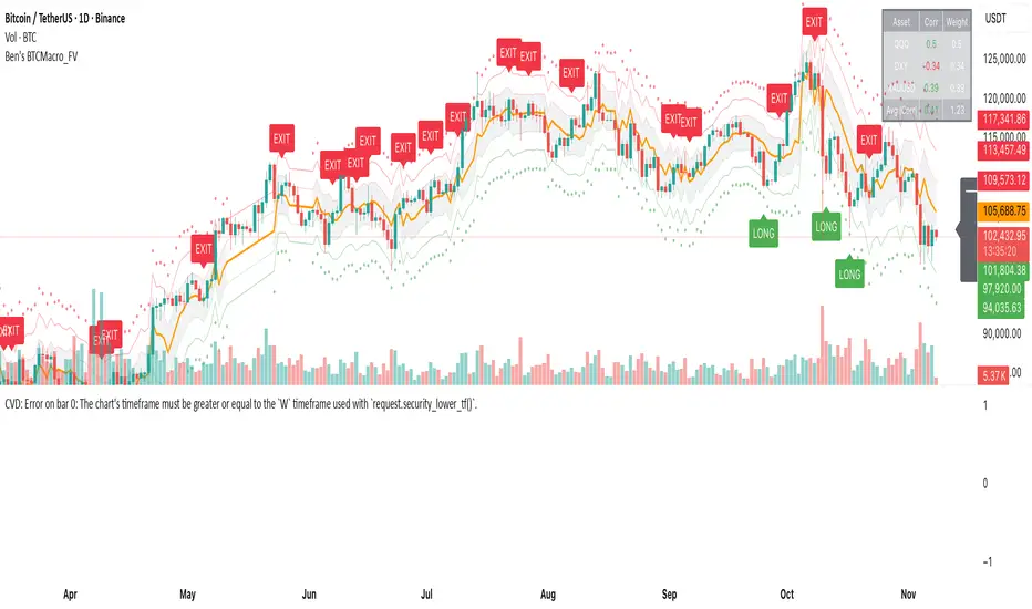
Sunmool's NY Lunch Model BacktestingICT NY Lunch Model Backtesting (12:00–13:00 NY) 🗽🍔
This research indicator tests an ICT narrative using the New York lunch window (12:00–13:00 America/New_York). It records that hour’s high/low and measures, during the post-lunch session (default 13:00–16:00), how often:
⬆️ If the afternoon trends up, the Lunch Low gets swept first.
⬇️ If the afternoon trends down, the Lunch High gets swept first.
It reports these as conditional probabilities, not trade signals. 📈
👀 What it shows
🟦 Lunch Range box (toggle): high/low from 12:00–13:00 NY
🔻🔺 Sweep signals (bar-anchored)
Low sweep: triangle below bar + optional “L”
High sweep: triangle above bar + optional “H”
🧱 Optional small box wrapping the swept candle
📊 Stats table (top-right)
P(L-swept | Up) — % of Up-days where Lunch Low was swept
P(H-swept | Down) — % of Down-days where Lunch High was swept
🔁 Contradictions + sample sizes (Up-days / Down-days)
🎯 Direction logic (Up/Down)
Anchor: 13:00 open (pmOpen) ⏰
Threshold: ATR × multiple or % from 13:00
Close ≥ pmOpen + threshold → Up-day
Close ≤ pmOpen − threshold → Down-day
Tiny moves under the threshold are ignored to reduce noise 🧹
⚙️ Inputs
🌐 Timezone: America/New_York (DST handled)
🍽️ Lunch window: 1200–1300
🕓 Post-lunch window: default 1300–1600 (try 17:00/20:00 for sensitivity)
📐 Trend threshold: ATR / Percent (with length/multiple or % level)
📅 Weekdays-only toggle (FX/Equities style)
👁️ Display toggles: Lunch box / sweep arrows / sweep text / sweep candle box / stats table
🔔 TF hint when chart TF > 15m
🧭 How to use
Use 5–15m charts for accurate lunch range capture.
Scroll ~1 year for meaningful samples.
Run sensitivity checks: vary ATR/% thresholds and the post-lunch end time.
For crypto, compare with vs without weekends. 🚀
🧠 Reading the results
High P(L-swept | Up) with a solid Up-day count ⇒ on up afternoons, lunch low is often swept.
High P(H-swept | Down) ⇒ on down afternoons, lunch high is often swept.
Lower Contradictions = cleaner tendency.
Remember: this is a probabilistic tendency, not a rule. 🎲
📝 Notes & limits
All markers (arrows, text, sweep boxes) are bar-anchored; the lunch range box is a research overlay you can toggle.
Real-time vs historical bar building can differ—interpret on bar close. 🔒

Time Period Highlighter (UTC) — SPARTANHighlights sessions
00:00 UTC - 06:00 UTC
06:00 UTC - 12:00 UTC
12:00 UTC - 12:00 UTC

4-Hour Range Scalping [v6.3]User Guide: 4-Hour Range Scalping Strategy
Hello! Here is the guide for the Pine Script strategy. Please read it carefully to get the best results.
📈 This script automates the "4-Hour Range Scalping Strategy" from the video.
The main idea is that the first four hours of a major trading day (like New York) set up a "trap zone." The strategy waits for the price to break out of this zone and then fail, giving us a signal that the breakout was false and the price is likely to reverse.
Here’s the simple logic:
Define the Range: It precisely calculates the highest high and lowest low during the first four hours of the selected trading session (e.g., 00:00 to 04:00 New York Time).
Wait for a Breakout: It then monitors the 5-minute chart for a price breakout where a candle fully closes outside of this established range.
Identify the Reversal: The trade trigger occurs when the price fails to continue its breakout and a subsequent 5-minute candle closes back inside the range. This signals a potential reversal or "failed breakout."
Execute the Trade:
]A Short (Sell) trade is triggered after a failed breakout above the range high.
A Long (Buy) trade is triggered after a failed breakout below the range low.
Manage the Risk: The Stop Loss is automatically placed at the peak (for shorts) or trough (for longs) of the breakout move, and the Take Profit is set to a default 2:1 Risk/Reward Ratio.
How to Use the Script (Step-by-Step) ⚙️
Follow these instructions to get it running perfectly.
1. Set Your Chart Timeframe This is the most important step. The strategy is designed to run on a 5-minute (5m) chart. Open your TradingView chart and make sure the timeframe is set to "5m".
2. Add the Script to Your Chart Open the Pine Editor tab at the bottom of TradingView, paste the entire script, and click the "Add to chart" button.
3. Configure the Settings On your chart, find the strategy's name (e.g., "4-Hour Range Scalping ") and click the gear icon ⚙️ to open its settings.
Trading Session: Choose the session for the range. New York is the default and the one from the video.
Risk/Reward Ratio: The default is 2.0, meaning your potential profit is twice your potential loss. You can adjust this to test other targets.
Backtesting Period: To see how the strategy performed on all historical data, go to the "Strategy Tester" panel, click its own gear icon ⚙️, and uncheck the boxes for "Start Date" and "End Date."
4. Understand the Visuals on Your Chart
Blue Background Area: This is the 4-hour calculation window. The script is identifying the day's high and low during this time. No trades will ever happen here.
Red Line (Range High): The highest price of the 4-hour window. This is the upper boundary of the "trap zone."
Green Line (Range Low): The lowest price of the 4-hour window. This is the lower boundary.
Green Triangle (▲): Shows where a Long (Buy) trade was entered.
Red Triangle (▼): Shows where a Short (Sell) trade was entered.
A Very Important Note on Timezones 🕒
This is critical for you in the Philippines (PHT).
The script is based on the New York session, which is 12 hours behind you. Your TradingView chart will still show your local time, but the script works on NY time in the background.
The New York "day" begins at 12:00 PM (Noon) your time.
The script's blue calculation window will be from 12:00 PM to 4:00 PM your local time.
The red and green range lines will appear on your chart only after 4:00 PM your time.
So, if you look at your chart in the morning or early afternoon, you will not see today's range yet. This is normal! The script is just waiting for the New York session to start.
How to Set Up Trade Alerts 🔔
You can have TradingView send you a notification whenever the script enters a trade.
Click the "Alert" button (looks like a clock) in the right-hand toolbar of TradingView.
In the "Condition" dropdown, select the name of the script (e.g., "4-Hour Range Scalping...").
You will then see two options: "Long Signal" and "Short Signal".
Select one (e.g., "Long Signal") and configure how you want to be notified (e.g., "Notify on app").
Click "Create". Repeat the process to create an alert for the other signal.
⚠️ Important Disclosure
For Educational and Research Purposes Only.
This script and all accompanying information are provided for educational and research purposes only. The strategy demonstrated is a technical concept and should not be misconstrued as financial, investment, legal, or tax advice.
Trading financial markets involves substantial risk and is not suitable for every investor. There is a possibility that you could sustain a loss of some or all of your initial investment. Therefore, you should not invest money that you cannot afford to lose.
Past performance is not indicative of future results. The backtesting results shown by this script are historical and do not guarantee future performance. Market conditions are constantly changing.
By using this script, you acknowledge that you are solely responsible for any and all trading decisions you make. You should conduct your own thorough research and, if necessary, seek advice from an independent financial advisor before making any investment decisions. The creators of this script assume no liability for any of your trading results.

多周期趋势动量面板加强版(Multi-Timeframe Trend Momentum Panel - User Guide)多周期趋势动量面板(Multi-Timeframe Trend Momentum Panel - User Guide)(english explanation follows.)
📖 指标功能详解 (精简版):
🎯 核心功能:
1. 多周期趋势分析 同时监控8个时间周期(1m/5m/15m/1H/4H/D/W/M)
2. 4维度投票系统 MA趋势+RSI动量+MACD+布林带综合判断
3. 全球交易时段 可视化亚洲/伦敦/纽约交易时间
4. 趋势强度评分 0100%量化市场力量
5. 智能警报 强势多空信号自动推送
________________________________________
📚 重要名词解释:
🔵 趋势状态 (MA均线分析):
名词 含义 信号强度
强势多头 快MA远高于慢MA(差值≥0.35%) ⭐⭐⭐⭐⭐ 做多
多头倾向 快MA略高于慢MA(差值<0.35%) ⭐⭐⭐ 谨慎做多
震荡 快慢MA缠绕,无明确方向 ⚠️ 观望
空头倾向 快MA略低于慢MA ⭐⭐⭐ 谨慎做空
强势空头 快MA远低于慢MA ⭐⭐⭐⭐⭐ 做空
简单理解: 快MA就像短跑运动员(反应快),慢MA是长跑运动员(稳定)。短跑远超长跑=强势多头,反之=强势空头。
________________________________________
🟠 动量状态 (RSI力度分析):
名词 含义 操作建议
动量上攻↗ RSI>60且快速上升 强烈买入信号
动量高位 RSI>60但上升变慢 警惕回调,可减仓
动量中性 RSI在4060之间,平稳 等待方向明确
动量低位 RSI<40但下跌变慢 警惕反弹,可止盈
动量下压↘ RSI<40且快速下降 强烈卖出信号
简单理解: RSI就像汽车速度表。"动量上攻"=油门踩到底加速,"动量高位"=已经很快但不再加速了。
________________________________________
🟣 辅助信号:
MACD:
• MACD多头 = 柱状图>0 = 买方力量强
• MACD空头 = 柱状图<0 = 卖方力量强
布林带(BB):
• BB超买 = 价格在布林带上轨附近 = 可能回调
• BB超卖 = 价格在布林带下轨附近 = 可能反弹
• BB中轨 = 价格在中间位置 = 平衡状态
________________________________________
💡 快速上手 3步看懂面板:
第1步: 看"综合结论标签" (K线上方)
• 绿色"多头占优" → 可以做多
• 红色"空头占优" → 可以做空
• 橙色"震荡/均衡" → 观望
第2步: 看"票数 多/空" (面板最下方)
• 多头票数远大于空头 (差距>2) → 趋势强
• 票数接近 (差距<1) → 震荡市
第3步: 看"趋势强度" (综合标签中)
• 强度>70% → 强势趋势,可重仓
• 强度5070% → 中等趋势,正常仓位
• 强度<50% → 弱势,轻仓或观望
________________________________________
🎨 时段背景色含义:
• 紫色背景 = 亚洲时段 (东京交易时间) 波动较小
• 橙色背景 = 伦敦时段 (欧洲交易时间) 波动增大
• 蓝色背景 = 纽约凌晨 美盘准备阶段
• 红色背景 = 纽约关键5分钟 (09:3009:35) ⚠️ 最重要! 市场最活跃,趋势易形成
• 绿色背景 = 纽约上午后段 延续早盘趋势
交易建议: 重点关注红色关键时段,这5分钟往往决定全天方向!
________________________________________
⚙️ 三大市场推荐设置
🥇 黄金: Hull MA 12/EMA 34, 阈值0.250.35%
₿ 比特币: EMA 21/EMA 55, 阈值0.801.20%
💎 以太坊: TEMA 21/EMA 55, 阈值0.600.80%
参数优化建议
黄金 (XAUUSD)
快速MA: Hull MA 12 (超灵敏捕捉黄金快速波动)
慢速MA: EMA 34 (斐波那契数列)
RSI周期: 9 (加快反应)
强趋势阈值: 0.25%
周期: 5, 15, 60, 240, 1440
比特币 (BTCUSD)
快速MA: EMA 21
慢速MA: EMA 55
RSI周期: 14
强趋势阈值: 0.8% (波动大,阈值需提高)
周期: 15, 60, 240, D, W
外汇 EUR/USD
快速MA: TEMA 10 (快速响应)
慢速MA: T3 30, 因子0.7 (平滑噪音)
RSI周期: 14
强趋势阈值: 0.08% (外汇波动小)
周期: 5, 15, 60, 240, 1440
📖 Indicator Function Details (Concise Version):
🎯 Core Functions:
1. MultiTimeframe Trend Analysis Monitors 8 timeframes simultaneously (1m/5m/15m/1H/4H/D/W/M)
2. 4Dimensional Voting System Comprehensive judgment based on MA trend + RSI momentum + MACD + Bollinger Bands
3. Global Trading Sessions Visualizes Asia/London/New York trading hours
4. Trend Strength Score Quantifies market strength from 0100%
5. Smart Alerts Automatically pushes strong bullish/bearish signals
📚 Key Term Explanations:
🔵 Trend Status (MA Analysis):
| Term | Meaning | Signal Strength |
| | | |
| Strong Bull | Fast MA significantly > Slow MA (Diff ≥0.35%) | ⭐⭐⭐⭐⭐ Long |
| Bullish Bias | Fast MA slightly > Slow MA (Diff <0.35%) | ⭐⭐⭐ Caution Long |
| Ranging | MAs intertwined, no clear direction | ⚠️ Wait & See |
| Bearish Bias | Fast MA slightly < Slow MA | ⭐⭐⭐ Caution Short |
| Strong Bear | Fast MA significantly < Slow MA | ⭐⭐⭐⭐⭐ Short |
Simple Understanding: Fast MA = sprinter (fast reaction), Slow MA = longdistance runner (stable). Sprinter far ahead = Strong Bull, opposite = Strong Bear.
🟠 Momentum Status (RSI Analysis):
| Term | Meaning | Trading Suggestion |
| | | |
| Momentum Up ↗ | RSI >60 & rising rapidly | Strong Buy Signal |
| Momentum High | RSI >60 but rising slower | Watch for pullback, consider reducing position |
| Momentum Neutral | RSI between 4060, stable | Wait for clearer direction |
| Momentum Low | RSI <40 but falling slower | Watch for rebound, consider taking profit |
| Momentum Down ↘ | RSI <40 & falling rapidly | Strong Sell Signal |
Simple Understanding: RSI = car speedometer. "Momentum Up" = full throttle acceleration, "Momentum High" = already fast but not accelerating further.
🟣 Auxiliary Signals:
MACD:
MACD Bullish = Histogram >0 = Strong buyer power
MACD Bearish = Histogram <0 = Strong seller power
Bollinger Bands (BB):
BB Overbought = Price near upper band = Possible pullback
BB Oversold = Price near lower band = Possible rebound
BB Middle = Price near middle band = Balanced state
💡 Quick Start 3 Steps to Understand the Panel:
Step 1: Check "Composite Conclusion Label" (Above the chart)
Green "Bulls Favored" → Consider Long
Red "Bears Favored" → Consider Short
Orange "Ranging/Balanced" → Wait & See
Step 2: Check "Votes Bull/Bear" (Bottom of the panel)
Bull votes significantly > Bear votes (Difference >2) → Strong Trend
Votes close (Difference <1) → Ranging Market
Step 3: Check "Trend Strength" (In the composite label)
Strength >70% → Strong Trend, consider heavier position
Strength 5070% → Moderate Trend, normal position size
Strength <50% → Weak Trend, light position or wait & see
🎨 Trading Session Background Color Meanings:
Purple = Asian Session (Tokyo hours) Lower volatility
Orange = London Session (European hours) Increased volatility
Blue = NY Early Morning US session preparation phase
Red = NY Critical 5 Minutes (09:3009:35) ⚠️ Most Important! Market most active, trends easily form
Green = NY Late Morning Continuation of early session trend
Trading Tip: Focus on the red critical period; these 5 minutes often determine the day's direction!
⚙️ Recommended Settings for Three Major Markets
🥇 Gold (XAUUSD):
Fast MA: Hull MA 12 (Highly sensitive for gold's fast moves)
Slow MA: EMA 34 (Fibonacci number)
RSI Period: 9 (Faster reaction)
Strong Trend Threshold: 0.25%
Timeframes: 5, 15, 60, 240, 1440
₿ Bitcoin (BTCUSD):
Fast MA: EMA 21
Slow MA: EMA 55
RSI Period: 14
Strong Trend Threshold: 0.8% (High volatility, requires higher threshold)
Timeframes: 15, 60, 240, D, W
💎 Ethereum (ETHUSD):
Fast MA: TEMA 21
Slow MA: EMA 55
RSI Period: 14
Strong Trend Threshold: 0.600.80%
Timeframes: 15, 60, 240, D, W
💱 Forex EUR/USD:
Fast MA: TEMA 10 (Fast response)
Slow MA: T3 30, Factor 0.7 (Smooths noise)
RSI Period: 14
Strong Trend Threshold: 0.08% (Forex has low volatility)
Timeframes: 5, 15, 60, 240, 1440
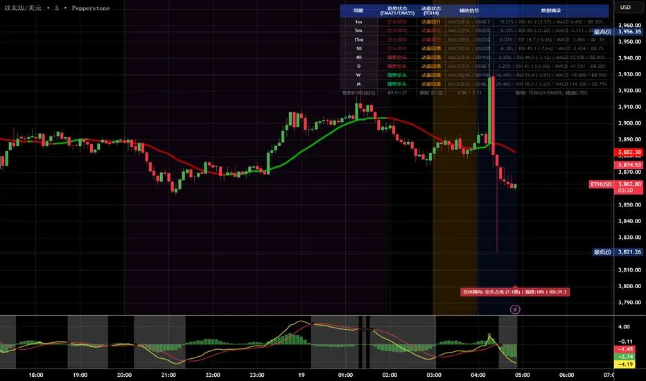
多周期趋势动量面板(Multi-Timeframe Trend Momentum Panel - User Guide)多周期趋势动量面板(Multi-Timeframe Trend Momentum Panel - User Guide)(english explanation follows.)
📖 指标功能详解 (精简版):
🎯 核心功能:
1. 多周期趋势分析 同时监控8个时间周期(1m/5m/15m/1H/4H/D/W/M)
2. 4维度投票系统 MA趋势+RSI动量+MACD+布林带综合判断
3. 全球交易时段 可视化亚洲/伦敦/纽约交易时间
4. 趋势强度评分 0100%量化市场力量
5. 智能警报 强势多空信号自动推送
________________________________________
📚 重要名词解释:
🔵 趋势状态 (MA均线分析):
名词 含义 信号强度
强势多头 快MA远高于慢MA(差值≥0.35%) ⭐⭐⭐⭐⭐ 做多
多头倾向 快MA略高于慢MA(差值<0.35%) ⭐⭐⭐ 谨慎做多
震荡 快慢MA缠绕,无明确方向 ⚠️ 观望
空头倾向 快MA略低于慢MA ⭐⭐⭐ 谨慎做空
强势空头 快MA远低于慢MA ⭐⭐⭐⭐⭐ 做空
简单理解: 快MA就像短跑运动员(反应快),慢MA是长跑运动员(稳定)。短跑远超长跑=强势多头,反之=强势空头。
________________________________________
🟠 动量状态 (RSI力度分析):
名词 含义 操作建议
动量上攻↗ RSI>60且快速上升 强烈买入信号
动量高位 RSI>60但上升变慢 警惕回调,可减仓
动量中性 RSI在4060之间,平稳 等待方向明确
动量低位 RSI<40但下跌变慢 警惕反弹,可止盈
动量下压↘ RSI<40且快速下降 强烈卖出信号
简单理解: RSI就像汽车速度表。"动量上攻"=油门踩到底加速,"动量高位"=已经很快但不再加速了。
________________________________________
🟣 辅助信号:
MACD:
• MACD多头 = 柱状图>0 = 买方力量强
• MACD空头 = 柱状图<0 = 卖方力量强
布林带(BB):
• BB超买 = 价格在布林带上轨附近 = 可能回调
• BB超卖 = 价格在布林带下轨附近 = 可能反弹
• BB中轨 = 价格在中间位置 = 平衡状态
________________________________________
💡 快速上手 3步看懂面板:
第1步: 看"综合结论标签" (K线上方)
• 绿色"多头占优" → 可以做多
• 红色"空头占优" → 可以做空
• 橙色"震荡/均衡" → 观望
第2步: 看"票数 多/空" (面板最下方)
• 多头票数远大于空头 (差距>2) → 趋势强
• 票数接近 (差距<1) → 震荡市
第3步: 看"趋势强度" (综合标签中)
• 强度>70% → 强势趋势,可重仓
• 强度5070% → 中等趋势,正常仓位
• 强度<50% → 弱势,轻仓或观望
________________________________________
🎨 时段背景色含义:
• 紫色背景 = 亚洲时段 (东京交易时间) 波动较小
• 橙色背景 = 伦敦时段 (欧洲交易时间) 波动增大
• 蓝色背景 = 纽约凌晨 美盘准备阶段
• 红色背景 = 纽约关键5分钟 (09:3009:35) ⚠️ 最重要! 市场最活跃,趋势易形成
• 绿色背景 = 纽约上午后段 延续早盘趋势
交易建议: 重点关注红色关键时段,这5分钟往往决定全天方向!
________________________________________
⚙️ 三大市场推荐设置
🥇 黄金: Hull MA 12/EMA 34, 阈值0.250.35%
₿ 比特币: EMA 21/EMA 55, 阈值0.801.20%
💎 以太坊: TEMA 21/EMA 55, 阈值0.600.80%
参数优化建议
黄金 (XAUUSD)
快速MA: Hull MA 12 (超灵敏捕捉黄金快速波动)
慢速MA: EMA 34 (斐波那契数列)
RSI周期: 9 (加快反应)
强趋势阈值: 0.25%
周期: 5, 15, 60, 240, 1440
比特币 (BTCUSD)
快速MA: EMA 21
慢速MA: EMA 55
RSI周期: 14
强趋势阈值: 0.8% (波动大,阈值需提高)
周期: 15, 60, 240, D, W
外汇 EUR/USD
快速MA: TEMA 10 (快速响应)
慢速MA: T3 30, 因子0.7 (平滑噪音)
RSI周期: 14
强趋势阈值: 0.08% (外汇波动小)
周期: 5, 15, 60, 240, 1440
📖 Indicator Function Details (Concise Version):
🎯 Core Functions:
1. MultiTimeframe Trend Analysis Monitors 8 timeframes simultaneously (1m/5m/15m/1H/4H/D/W/M)
2. 4Dimensional Voting System Comprehensive judgment based on MA trend + RSI momentum + MACD + Bollinger Bands
3. Global Trading Sessions Visualizes Asia/London/New York trading hours
4. Trend Strength Score Quantifies market strength from 0100%
5. Smart Alerts Automatically pushes strong bullish/bearish signals
📚 Key Term Explanations:
🔵 Trend Status (MA Analysis):
| Term | Meaning | Signal Strength |
| | | |
| Strong Bull | Fast MA significantly > Slow MA (Diff ≥0.35%) | ⭐⭐⭐⭐⭐ Long |
| Bullish Bias | Fast MA slightly > Slow MA (Diff <0.35%) | ⭐⭐⭐ Caution Long |
| Ranging | MAs intertwined, no clear direction | ⚠️ Wait & See |
| Bearish Bias | Fast MA slightly < Slow MA | ⭐⭐⭐ Caution Short |
| Strong Bear | Fast MA significantly < Slow MA | ⭐⭐⭐⭐⭐ Short |
Simple Understanding: Fast MA = sprinter (fast reaction), Slow MA = longdistance runner (stable). Sprinter far ahead = Strong Bull, opposite = Strong Bear.
🟠 Momentum Status (RSI Analysis):
| Term | Meaning | Trading Suggestion |
| | | |
| Momentum Up ↗ | RSI >60 & rising rapidly | Strong Buy Signal |
| Momentum High | RSI >60 but rising slower | Watch for pullback, consider reducing position |
| Momentum Neutral | RSI between 4060, stable | Wait for clearer direction |
| Momentum Low | RSI <40 but falling slower | Watch for rebound, consider taking profit |
| Momentum Down ↘ | RSI <40 & falling rapidly | Strong Sell Signal |
Simple Understanding: RSI = car speedometer. "Momentum Up" = full throttle acceleration, "Momentum High" = already fast but not accelerating further.
🟣 Auxiliary Signals:
MACD:
MACD Bullish = Histogram >0 = Strong buyer power
MACD Bearish = Histogram <0 = Strong seller power
Bollinger Bands (BB):
BB Overbought = Price near upper band = Possible pullback
BB Oversold = Price near lower band = Possible rebound
BB Middle = Price near middle band = Balanced state
💡 Quick Start 3 Steps to Understand the Panel:
Step 1: Check "Composite Conclusion Label" (Above the chart)
Green "Bulls Favored" → Consider Long
Red "Bears Favored" → Consider Short
Orange "Ranging/Balanced" → Wait & See
Step 2: Check "Votes Bull/Bear" (Bottom of the panel)
Bull votes significantly > Bear votes (Difference >2) → Strong Trend
Votes close (Difference <1) → Ranging Market
Step 3: Check "Trend Strength" (In the composite label)
Strength >70% → Strong Trend, consider heavier position
Strength 5070% → Moderate Trend, normal position size
Strength <50% → Weak Trend, light position or wait & see
🎨 Trading Session Background Color Meanings:
Purple = Asian Session (Tokyo hours) Lower volatility
Orange = London Session (European hours) Increased volatility
Blue = NY Early Morning US session preparation phase
Red = NY Critical 5 Minutes (09:3009:35) ⚠️ Most Important! Market most active, trends easily form
Green = NY Late Morning Continuation of early session trend
Trading Tip: Focus on the red critical period; these 5 minutes often determine the day's direction!
⚙️ Recommended Settings for Three Major Markets
🥇 Gold (XAUUSD):
Fast MA: Hull MA 12 (Highly sensitive for gold's fast moves)
Slow MA: EMA 34 (Fibonacci number)
RSI Period: 9 (Faster reaction)
Strong Trend Threshold: 0.25%
Timeframes: 5, 15, 60, 240, 1440
₿ Bitcoin (BTCUSD):
Fast MA: EMA 21
Slow MA: EMA 55
RSI Period: 14
Strong Trend Threshold: 0.8% (High volatility, requires higher threshold)
Timeframes: 15, 60, 240, D, W
💎 Ethereum (ETHUSD):
Fast MA: TEMA 21
Slow MA: EMA 55
RSI Period: 14
Strong Trend Threshold: 0.600.80%
Timeframes: 15, 60, 240, D, W
💱 Forex EUR/USD:
Fast MA: TEMA 10 (Fast response)
Slow MA: T3 30, Factor 0.7 (Smooths noise)
RSI Period: 14
Strong Trend Threshold: 0.08% (Forex has low volatility)
Timeframes: 5, 15, 60, 240, 1440

Mark the New York trading session hours(纽约交易时间段标注)Apply background shading for New York time.
(纽约时间背景着色)
04:00 ~ 09:00
09:00 ~ 09:30
09:30 ~ 12:00
No shading needed after 12 AM as I'll be asleep.
(12点我睡觉了就不着色了。)
ALMASTO – Pro Trend & Momentum (v1.1)ALMASTO — Pro Trend & Momentum Strategy
Description:
This strategy is designed for precision trading in both Forex (FX) and Crypto markets.
It combines multi-timeframe trend confirmation (EMA200), momentum filters (RSI, MACD, ADX), and ATR-based dynamic risk management.
ALMASTO — Pro Trend & Momentum Strategy automatically manages take-profit levels, stop-loss, and breakeven adjustments once TP1 is reached — providing a structured and emotion-free trading approach.
Optimal Use
Works best on lower timeframes (5m–15m) with strong liquidity sessions.
Optimized for pairs like EURUSD, XAUUSD, and BTCUSDT.
Built for trend-following setups and momentum reversals with high volatility confirmation.
Recommended Settings
🔹 Forex – 5m
EMA Fast = 34, EMA Slow = 200, HTF = 1H
RSI (14): Long ≥ 55 / Short ≤ 45
MACD (8 / 21 / 5), ADX Len 10 / Min 27
ATR Len 7, Stop Loss = ATR × 2.1
TP1 = 1.1 RR, TP2 = 2.3 RR
Session = 07:00–11:00 & 12:30–16:00 (Exchange Time)
Risk = 0.8% per trade
🔹 Forex – 15m
EMA Fast = 50, EMA Slow = 200, HTF = 4H
RSI (14): Long ≥ 53 / Short ≤ 47
MACD (12 / 26 / 9), ADX Min 24
ATR Len 10, SL = ATR × 1.9
TP1 = 1.2 RR, TP2 = 2.6 RR
Risk = 1.0% per trade
🔹 Crypto – 5m (BTC/USDT)
EMA Fast = 34, EMA Slow = 200, HTF = 4H
RSI (14): Long ≥ 56 / Short ≤ 44
MACD (8 / 21 / 5), ADX Min 30
ATR Len 7, SL = ATR × 2.2
TP1 = 1.0 RR, TP2 = 2.5 RR
Session = 00:00–06:00 & 12:00–22:00 (UTC)
Risk = 0.5% per trade
Core Features
✅ Auto breakeven after TP1
✅ Dual take-profit system (1:1 & 1:2 RR)
✅ ATR-based stop & trailing logic
✅ Filters for session time, volume, and volatility
✅ Candle-body vs ATR size filter to avoid noise
✅ Optional cooldown between trades
Important Notes
Use bar close confirmation only (barstate.isconfirmed) to avoid repainting on lower timeframes.
Adjust commission (0.01–0.03%) and slippage (1–2 ticks) in Strategy Tester for realistic results.
Avoid low-liquidity hours (after 21:00 UTC for FX / after midnight for crypto).
Backtest using realistic broker data (e.g., BlackBull Markets / Bybit / Binance Futures).
Best results occur during London & New York sessions with moderate volatility.
⚠️ Disclaimer
This script is for educational and research purposes only.
It does not constitute financial advice.
Use proper risk management and test thoroughly before using on live accounts.
Developed by KING FX Labs
Built and optimized by Yousef Almasto — combining advanced price-action logic, multi-timeframe EMA structure, and volatility-adaptive ATR management.
Tested across Forex, Gold, and Crypto markets to ensure consistent performance and minimal drawdown.
📈 “Precision Trading. Zero Emotion. Pure Momentum.”

Volume Bubbles & Liquidity Heatmap [LuxAlgo]The Volume Bubbles & Liquidity Heatmap indicator highlights volume and liquidity clearly and precisely with its volume bubbles and liquidity heat map, allowing to identify key price areas.
Customize the bubbles with different time frames and different display modes: total volume, buy and sell volume, or delta volume.
🔶 USAGE
The primary objective of this tool is to offer traders a straightforward method for analyzing volume on any selected timeframe.
By default, the tool displays buy and sell volume bubbles for the daily timeframe over the last 2,000 bars. Traders should be aware of the difference between the timeframe of the chart and that of the bubbles.
The tool also displays a liquidity heat map to help traders identify price areas where liquidity accumulates or is lacking.
🔹 Volume Bubbles
The bubbles have three possible display modes:
Total Volume: Displays the total volume of trades per bubble.
Buy & Sell Volume: Each bubble is divided into buy and sell volume.
Delta Volume: Displays the difference between buy and sell volume.
Each bubble represents the trading volume for a given period. By default, the timeframe for each bubble is set to daily, meaning each bubble represents the trading volume for each day.
The size of each bubble is proportional to the volume traded; a larger bubble indicates greater volume, while a smaller bubble indicates lower volume.
The color of each bubble indicates the dominant volume: green for buy volume and red for sell volume.
One of the tool's main goals is to facilitate simple, clear, multi-timeframe volume analysis.
The previous chart shows Delta Volume bubbles with various chart and bubble timeframe configurations.
To correctly visualize the bubbles, traders must ensure there is a sufficient number of bars per bubble. This is achieved by using a lower chart timeframe and a higher bubble timeframe.
As can be seen in the image above, the greater the difference between the chart and bubble timeframes, the better the visualization.
🔹 Liquidity Heatmap
The other main element of the tool is the liquidity heatmap. By default, it divides the chart into 25 different price areas and displays the accumulated trading volume on each.
The image above shows a 4-hour BTC chart displaying only the liquidity heatmap. Traders should be aware of these key price areas and observe how the price behaves in them, looking for possible opportunities to engage with the market.
The main parameters for controlling the heatmap on the settings panel are Rows and Cell Minimum Size. Rows modifies the number of horizontal price areas displayed, while Cell Minimum Size modifies the minimum size of each liquidity cell in each row.
As can be seen in the above BTC hourly chart, the cell size is 24 at the top and 168 at the bottom. The cells are smaller on top and bigger on the bottom.
The color of each cell reflects the liquidity size with a gradient; this reflects the total volume traded within each cell. The default colors are:
Red: larger liquidity
Yellow: medium liquidity
Blue: lower liquidity
🔹 Using Both Tools Together
This indicator provides the means to identify directional bias and market timing.
The main idea is that if buyers are strong, prices are likely to increase, and if sellers are strong, prices are likely to decrease. This gives us a directional bias for opening long or short positions. Then, we combine our directional bias with price rejection or acceptance of key liquidity levels to determine the timing of opening or closing our positions.
Now, let's review some charts.
This first chart is BTC 1H with Delta Weekly Bubbles. Delta Bubbles measure the difference between buy and sell volume, so we can easily see which group is dominant (buyers or sellers) and how strong they are in any given week. This, along with the key price areas displayed by the Liquidity Heatmap, can help us navigate the markets.
We divided market behavior into seven groups, and each group has several bubbles, numbered from 1 to 17.
Bubbles 1, 2, and 3: After strong buyers market consolidates with positive delta, prices move up next week.
Bubbles 3, 4, and 5: Strength changes from buyers to sellers. Next week, prices go down.
Bubbles 6 and 7: The market trades at higher prices, but with negative delta. Next week, prices go down.
Bubbles 7, 8, and 9: Strength changes from sellers to buyers. Next weeks (9 and 10), prices go up.
Bubbles 10, 11, and 12: After strong buyers prices trade higher with a negative delta. Next weeks (12 and 13) prices go down.
Bubbles 12, 14, and 15: Strength changes from sellers to buyers; next week, prices increase.
Bubbles 15 and 16: The market trades higher with a very small positive delta; next week, prices go down.
Current bubble/week 17 is not yet finished. Right now, it is trading lower, but with a smaller negative delta than last week. This may signal that sellers are losing strength and that a potential reversal will follow, with prices trading higher.
This is the same BTC 1H chart, but with price rejections from key liquidity areas acting as strong price barriers.
When prices reach a key area with strong liquidity and are rejected, it signals a good time to take action.
By observing price behavior at certain key price levels, we can improve our timing for entering or exiting the markets.
🔶 DETAILS
🔹 Bubbles Display
From the settings panel, traders can configure the bubbles with four main parameters: Mode, Timeframe, Size%, and Shape.
The image above shows five-minute BTC charts with execution over the last 3,500 bars, different display modes, a daily timeframe, 100% size, and shape one.
The Size % parameter controls the overall size of the bubbles, while the Shape parameter controls their vertical growth.
Since the chart has two scales, one for time and one for price, traders can use the Shape parameter to make the bubbles round.
The chart above shows the same bubbles with different size and shape parameters.
You can also customize data labels and timeframe separators from the settings panel.
🔶 SETTINGS
Execute on last X bars: Number of bars for indicator execution
🔹 Bubbles
Display Bubbles: Enable/Disable volume bubbles.
Bubble Mode: Select from the following options: total volume, buy and sell volume, or the delta between buy and sell volume.
Bubble Timeframe: Select the timeframe for which the bubbles will be displayed.
Bubble Size %: Select the size of the bubbles as a percentage.
Bubble Shape: Select the shape of the bubbles. The larger the number, the more vertical the bubbles will be stretched.
🔹 Labels
Display Labels: Enable/Disable data labels, select size and location.
🔹 Separators
Display Separators: Enable/Disable timeframe separators and select color.
🔹 Liquidity Heatmap
Display Heatmap: Enable/Disable liquidity heatmap.
Heatmap Rows: select number of rows to be displayed.
Cell Minimum Size: Select the minimum size for each cell in each row.
Colors.
🔹 Style
Buy & Sell Volume Colors.

Hilly's Advanced Crypto Scalping Strategy - 5 Min ChartTo determine the "best" input parameters for the Advanced Crypto Scalping Strategy on a 5-minute chart, we need to consider the goals of optimizing for profitability, minimizing false signals, and adapting to the volatile nature of cryptocurrencies. The default parameters in the script are a starting point, but the optimal values depend on the specific cryptocurrency pair, market conditions, and your risk tolerance. Below, I'll provide recommended input values based on common practices in crypto scalping, along with reasoning for each parameter. I’ll also suggest how to fine-tune them using TradingView’s backtesting and optimization tools.
Recommended Input Parameters
These values are tailored for a 5-minute chart for liquid cryptocurrencies like BTC/USD or ETH/USD on exchanges like Binance or Coinbase. They aim to balance signal frequency and accuracy for day trading.
Fast EMA Length (emaFastLen): 9
Reasoning: A 9-period EMA is commonly used in scalping to capture short-term price movements while remaining sensitive to recent price action. It reacts faster than the default 10, aligning with the 5-minute timeframe.
Slow EMA Length (emaSlowLen): 21
Reasoning: A 21-period EMA provides a good balance for identifying the broader trend on a 5-minute chart. It’s slightly longer than the default 20 to reduce noise while confirming the trend direction.
RSI Length (rsiLen): 14
Reasoning: The default 14-period RSI is a standard choice for momentum analysis. It works well for detecting overbought/oversold conditions without being too sensitive on short timeframes.
RSI Overbought (rsiOverbought): 75
Reasoning: Raising the overbought threshold to 75 (from 70) reduces false sell signals in strong bullish trends, which are common in crypto markets.
RSI Oversold (rsiOversold): 25
Reasoning: Lowering the oversold threshold to 25 (from 30) filters out weaker buy signals, ensuring entries occur during stronger reversals.
MACD Fast Length (macdFast): 12
Reasoning: The default 12-period fast EMA for MACD is effective for capturing short-term momentum shifts in crypto, aligning with scalping goals.
MACD Slow Length (macdSlow): 26
Reasoning: The default 26-period slow EMA is a standard setting that works well for confirming momentum trends without lagging too much.
MACD Signal Smoothing (macdSignal): 9
Reasoning: The default 9-period signal line is widely used and provides a good balance for smoothing MACD crossovers on a 5-minute chart.
Bollinger Bands Length (bbLen): 20
Reasoning: The default 20-period Bollinger Bands are effective for identifying volatility breakouts, which are key for scalping in crypto markets.
Bollinger Bands Multiplier (bbMult): 2.0
Reasoning: A 2.0 multiplier is standard and captures most price action within the bands. Increasing it to 2.5 could reduce signals but improve accuracy in highly volatile markets.
Stop Loss % (slPerc): 0.8%
Reasoning: A tighter stop loss of 0.8% (from 1.0%) suits the high volatility of crypto, helping to limit losses on false breakouts while keeping risk manageable.
Take Profit % (tpPerc): 1.5%
Reasoning: A 1.5% take-profit target (from 2.0%) aligns with scalping’s goal of capturing small, frequent gains. Crypto markets often see quick reversals, so a smaller target increases the likelihood of hitting profits.
Use Candlestick Patterns (useCandlePatterns): True
Reasoning: Enabling candlestick patterns (e.g., engulfing, hammer) adds confirmation to signals, reducing false entries in choppy markets.
Use Volume Filter (useVolumeFilter): True
Reasoning: The volume filter ensures signals occur during high-volume breakouts, which are more likely to sustain in crypto markets.
Signal Arrow Size (signalSize): 2.0
Reasoning: Increasing the arrow size to 2.0 (from 1.5) makes buy/sell signals more visible on the chart, especially on smaller screens or volatile price action.
Background Highlight Transparency (bgTransparency): 85
Reasoning: A slightly higher transparency (85 from 80) keeps the background highlights subtle but visible, avoiding chart clutter.
How to Apply These Parameters
Copy the Script: Use the Pine Script provided in the previous response.
Paste in TradingView: Open TradingView, go to the Pine Editor, paste the code, and click "Add to Chart."
Set Parameters: In the strategy settings, manually input the recommended values above or adjust them via the input fields.
Test on a 5-Minute Chart: Apply the strategy to a liquid crypto pair (e.g., BTC/USDT, ETH/USDT) on a 5-minute chart.
Fine-Tuning for Optimal Performance
To find the absolute best parameters for your specific trading pair and market conditions, use TradingView’s Strategy Tester and optimization features:
Backtesting:
Run the strategy on historical data for your chosen pair (e.g., BTC/USDT on Binance).
Check metrics like Net Profit, Profit Factor, Win Rate, and Max Drawdown in the Strategy Tester.
Focus on a sample period of at least 1–3 months to capture various market conditions (bull, bear, sideways).
Parameter Optimization:
In the Strategy Tester, click the settings gear next to the strategy name.
Enable optimization for key inputs like emaFastLen (test range: 7–12), emaSlowLen (15–25), slPerc (0.5–1.5), and tpPerc (1.0–3.0).
Run the optimization to find the combination with the highest net profit or best Sharpe ratio, but avoid over-optimization (curve-fitting) by testing on out-of-sample data.
Market-Specific Adjustments:
Volatile Pairs (e.g., DOGE/USDT): Use tighter stop losses (e.g., 0.5–0.7%) and smaller take-profit targets (e.g., 1.0–1.2%) to account for rapid price swings.
Stable Pairs (e.g., BTC/USDT): Slightly wider stop losses (e.g., 1.0–1.2%) and take-profit targets (e.g., 1.8–2.5%) may work better.
Trending Markets: Increase emaSlowLen (e.g., to 25–30) to follow stronger trends.
Choppy Markets: Tighten bbMult (e.g., to 1.8) and lower rsiOverbought/rsiOversold (e.g., to 70/30) to filter noise.
Forward Testing:
After backtesting, run the strategy in real-time on a demo account for 1–2 weeks to validate performance under current market conditions.
Important Notes
No Universal "Best" Numbers: Optimal parameters vary by crypto pair, exchange, and market conditions (e.g., bull vs. bear market). The suggested values are a starting point based on common scalping practices.
Risk Management: Never risk more than 1–2% of your account per trade. Adjust position sizing in TradingView’s strategy settings to align with your risk tolerance.
Market Volatility: Crypto markets are highly volatile. Test the strategy on your specific pair and adjust parameters if signals are too frequent or too rare.
Not Financial Advice: This is an educational tool. Backtest thoroughly and use a demo account before trading with real funds.
If you want me to generate a chart showing backtest performance for specific parameters or to tweak the script further (e.g., adding more indicators or adjusting signal logic), let me know!can you add clear buy ans sell signs above the candles in this codeTo add clear buy and sell signals above the candles in the provided Pine Script, I'll modify the existing code to include prominent text labels directly above (for sell signals) and below (for buy signals) the candles. These labels will be larger, color-coded, and positioned to avoid clutter, ensuring they are easily visible on the chart. The core strategy logic (EMA, RSI, MACD, Bollinger Bands, candlestick patterns, and volume filter) will remain unchanged, and I'll reuse the same artifact_id since this is an update to the previous script.AdvancedCryptoScalpingStrategy.pinex-pine

Sunset Zones by PDVDescription
Sunset Zones by PDV is an intraday reference indicator that plots key horizontal levels based on selected “root candles” throughout the trading day. At each programmed time, the indicator identifies the high and low of the corresponding candle and projects those levels forward with extended lines, providing traders with a clean visual framework of potential intraday reaction zones.
These zones serve as reference levels for support, resistance, liquidity grabs, and session context, allowing traders to analyze how price reacts around time-specific structures. Unlike lagging indicators, Sunset Zones gives traders real-time, rule-based levels tied directly to the price action of specific moments in the session.
Key Features
Predefined Time Codes
The script comes with a curated list of intraday timestamps (in HHMM format). Each represents a “root candle” from which levels are generated. Examples include 03:12, 06:47, 07:41, 08:51, etc. These time codes can reflect historically important market moments such as session opens, liquidity sweeps, or volatility inflection points.
Automatic Zone Plotting
At each root time, the script captures the candle’s high and low and instantly extends those levels forward across the chart. This provides consistent, objective reference points for intraday trading.
Extended Lines
Levels are projected far into the future (default: 500 bars) so traders can easily track how price interacts with those zones throughout the day.
Color-Coded Levels
Each root time is assigned a distinct color for fast identification. For example:
03:12 → Fuchsia
06:47 → Purple
07:41 → Teal
08:51 → White
09:53 → White
10:20 → Orange
11:10 → Green
11:49 → Red
12:05 → White
13:05 → Teal
14:09 → Aqua
This helps traders quickly recognize which time-of-day level price is interacting with.
Lightweight & Visual
The indicator focuses purely on price and time, avoiding complexity or lagging signals. It can be layered with other analysis tools, order flow charts, or session-based studies.
Practical Use Cases
Intraday Bias:
Observe whether price respects, rejects, or consolidates around these reference levels to form a bias.
Liquidity Zones:
High/low sweeps of the root candle can act as liquidity pools where institutions might trigger stops or reversals.
Support & Resistance:
Extended lines create intraday S/R zones without the need to manually draw levels.
Confluence Finder:
Combine Sunset Zones with VWAP, session ranges, Fibonacci levels, or higher-timeframe structure for layered confluence.
Important Notes
This is a visual reference tool only. It does not generate buy or sell signals.
Default times are provided, but the concept is flexible — traders can adapt it by modifying or expanding the list of time codes.
Works best on intraday timeframes where session structure is most relevant (e.g., 1-minute to 15-minute charts).
✅ In short: Sunset Zones by PDV gives intraday traders a systematic way to anchor their charts to important time-based highs and lows, creating a consistent framework for analyzing price reactions across the day.

FlowStateTrader FlowState Trader - Advanced Time-Filtered Strategy
## Overview
FlowState Trader is a sophisticated algorithmic trading strategy that combines precision entry signals with intelligent time-based filtering and adaptive risk management. Built for traders seeking to achieve their optimal performance state, FlowState identifies high-probability trading opportunities within user-defined time windows while employing dynamic trailing stops and partial position management.
## Core Strategy Philosophy
FlowState Trader operates on the principle that peak trading performance occurs when three elements align: **Focus** (precise entry signals), **Flow** (optimal time windows), and **State** (intelligent position management). This strategy excels at finding reversal opportunities at key support and resistance levels while filtering out suboptimal trading periods to keep traders in their optimal flow state.
## Key Features
### 🎯 Focus Entry System
**Support/Resistance Zone Trading**:
- Dynamic identification of key price levels using configurable lookback periods
- Entry signals triggered when price interacts with these critical zones
- Volume confirmation ensures genuine breakout/reversal momentum
- Trend filter alignment prevents counter-trend disasters
**Entry Conditions**:
- **Long Signals**: Price closes above support buffer, touches support level, with above-average volume
- **Short Signals**: Price closes below resistance buffer, touches resistance level, with above-average volume
- Optional trend filter using EMA or SMA for directional bias confirmation
### ⏰ FlowState Time Filtering System
**Comprehensive Time Controls**:
- **12-Hour Format Trading Windows**: User-friendly AM/PM time selection
- **Multi-Timezone Support**: UTC, EST, PST, CST with automatic conversion
- **Day-of-Week Filtering**: Trade only weekdays, weekends, or both
- **Lunch Hour Avoidance**: Automatically skips low-volume lunch periods (12-1 PM)
- **Visual Time Indicators**: Background coloring shows active/inactive trading periods
**Smart Time Features**:
- Handles overnight trading sessions seamlessly
- Prevents trades during historically poor performance periods
- Customizable trading hours for different market sessions
- Real-time trading window status in dashboard
### 🛡️ Adaptive Risk Management
**Multi-Level Take Profit System**:
- **TP1**: First profit target with optional partial position closure
- **TP2**: Final profit target for remaining position
- **Flexible Scaling**: Choose number of contracts to close at each level
**Dynamic Trailing Stop Technology**:
- **Three Operating Modes**:
- **Conservative**: Earlier activation, tighter trailing (protect profits)
- **Balanced**: Optimal risk/reward balance (recommended)
- **Aggressive**: Later activation, wider trailing (let winners run)
- **ATR-Based Calculations**: Adapts to current market volatility
- **Automatic Activation**: Engages when position reaches profitability threshold
### 📊 Intelligent Position Sizing
**Contract-Based Management**:
- Configurable entry quantity (1-1000 contracts)
- Partial close quantities for profit-taking
- Clear position tracking and P&L monitoring
- Real-time position status updates
### 🎨 Professional Visualization
**Enhanced Chart Elements**:
- **Entry Zone Highlighting**: Clear visual identification of trading opportunities
- **Dynamic Risk/Reward Lines**: Real-time TP and SL levels with price labels
- **Trailing Stop Visualization**: Live tracking of adaptive stop levels
- **Support/Resistance Lines**: Key level identification
- **Time Window Background**: Visual confirmation of active trading periods
**Dual Dashboard System**:
- **Strategy Dashboard**: Real-time position info, settings status, and current levels
- **Performance Scorecard**: Live P&L tracking, win rates, and trade statistics
- **Customizable Sizing**: Small, Medium, or Large display options
### ⚙️ Comprehensive Customization
**Core Strategy Settings**:
- **Lookback Period**: Support/resistance calculation period (5-100 bars)
- **ATR Configuration**: Period and multipliers for stops/targets
- **Reward-to-Risk Ratios**: Customizable profit target calculations
- **Trend Filter Options**: EMA/SMA selection with adjustable periods
**Time Filter Controls**:
- **Trading Hours**: Start/end times in 12-hour format
- **Timezone Selection**: Four major timezone options
- **Day Restrictions**: Weekend-only, weekday-only, or unrestricted
- **Session Management**: Lunch hour avoidance and custom periods
**Risk Management Options**:
- **Trailing Stop Modes**: Conservative/Balanced/Aggressive presets
- **Partial Close Settings**: Enable/disable with custom quantities
- **Alert System**: Comprehensive notifications for all trade events
### 📈 Performance Tracking
**Real-Time Metrics**:
- Net profit/loss calculation
- Win rate percentage
- Profit factor analysis
- Maximum drawdown tracking
- Total trade count and breakdown
- Current position P&L
**Trade Analytics**:
- Winner/loser ratio tracking
- Real-time performance scorecard
- Strategy effectiveness monitoring
- Risk-adjusted return metrics
### 🔔 Alert System
**Comprehensive Notifications**:
- Entry signal alerts with price and quantity
- Take profit level hits (TP1 and TP2)
- Stop loss activations
- Trailing stop engagements
- Position closure notifications
## Strategy Logic Deep Dive
### Entry Signal Generation
The strategy identifies high-probability reversal points by combining multiple confirmation factors:
1. **Price Action**: Looks for price interaction with key support/resistance levels
2. **Volume Confirmation**: Ensures sufficient market interest and liquidity
3. **Trend Alignment**: Optional filter prevents counter-trend positions
4. **Time Validation**: Only trades during user-defined optimal periods
5. **Zone Analysis**: Entry occurs within calculated buffer zones around key levels
### Risk Management Philosophy
FlowState Trader employs a three-tier risk management approach:
1. **Initial Protection**: ATR-based stop losses set at strategy entry
2. **Profit Preservation**: Trailing stops activate once position becomes profitable
3. **Scaled Exit**: Partial profit-taking allows for both security and potential
### Time-Based Edge
The time filtering system recognizes that not all trading hours are equal:
- Avoids low-volume, high-spread periods
- Focuses on optimal liquidity windows
- Prevents trading during news events (lunch hours)
- Allows customization for different market sessions
## Best Practices and Optimization
### Recommended Settings
**For Scalping (1-5 minute charts)**:
- Lookback Period: 10-20
- ATR Period: 14
- Trailing Stop: Conservative mode
- Time Filter: Major session hours only
**For Day Trading (15-60 minute charts)**:
- Lookback Period: 20-30
- ATR Period: 14-21
- Trailing Stop: Balanced mode
- Time Filter: Extended trading hours
**For Swing Trading (4H+ charts)**:
- Lookback Period: 30-50
- ATR Period: 21+
- Trailing Stop: Aggressive mode
- Time Filter: Disabled or very broad
### Market Compatibility
- **Forex**: Excellent for major pairs during active sessions
- **Stocks**: Ideal for liquid stocks during market hours
- **Futures**: Perfect for index and commodity futures
- **Crypto**: Effective on major cryptocurrencies (24/7 capability)
### Risk Considerations
- **Market Conditions**: Performance varies with volatility regimes
- **Timeframe Selection**: Lower timeframes require tighter risk management
- **Position Sizing**: Never risk more than 1-2% of account per trade
- **Backtesting**: Always test on historical data before live implementation
## Educational Value
FlowState serves as an excellent learning tool for:
- Understanding support/resistance trading
- Learning proper time-based filtering
- Mastering trailing stop techniques
- Developing systematic trading approaches
- Risk management best practices
## Disclaimer
This strategy is for educational and informational purposes only. Past performance does not guarantee future results. Trading involves substantial risk of loss and is not suitable for all investors. Users should thoroughly backtest the strategy and understand all risks before live trading. Always use proper position sizing and never risk more than you can afford to lose.
---
*FlowState Trader represents the evolution of systematic trading - combining classical technical analysis with modern risk management and intelligent time filtering to help traders achieve their optimal performance state through systematic, disciplined execution.*
