Fractal Resonance BarLazyBear's WaveTrend port has been praised for highlighting trend reversals with precision and punctuality (minimal lag). But strong "3rd Wave" trends can "embed" or saturate any oscillator flashing several premature crosses while stuck overbought/oversold. This happens when the trend stretches over a longer timescale than the oscillator's averaging window or filter time constant. Our solution: monitor many timescales. With Fractal Resonance Bar's rich color codings, strong wavefronts form across timescales and jump out like an approaching line of thunderclouds!
Fractal Resonance Bar color-codes the status of eight underlying stochastic oscillators, with each row averaging over twice the time of the row above.
Fractal Resonance Bar shifts its timescales along with your choice of main chart timescale:
1 minute chart: 1 minute through 128 minute (~2 hour) oscillators.
15 minute chart: 15 minute through 1920 minute (~32 hour) oscillators.
1 hour chart: 1 hour through 128 hour (~2 week) oscillators.
Daily chart: 1 day through 128 day (~4 month) oscillators.
The color map is configured as follows:
Hot Pink: Extreme Overbought (> 100%) rolled over to sell, but oscillators probably embedded with more upside (revert to Dark Green) possible after a pause.
Deep Red: Overbought (> 75%) crossover ripe for selling (validated when red spreads to timescales below).
Brown: Minor (< 75%) crossover sell from which could bounce back green or start a plunge toward gray/black.
Gray/Black: Mature (< -75%) sells turning full black in a plunge before the dawn.
Lime Green: Extreme Oversold (< -100%) and bouncing, though may yet bottom even lower.
Green: Oversold (< -75%) crossover ripe for buy. Green spreading to all timescales below will validate bottom is in.
Dark Green/Teal: Mature buy in overbought (> 75%) range, waiting for sell crossover to Hot Pink for a pause or correction.
White Stripes are Impulsive Trend Warning
Fractal Resonance Bar warns of oscillator embedding by showing white stripes when it detects strong, early surges in the timescale rows below.The white stripes usually accompany Hot Pink warning it's too early to go short, or Lime Green warning it's too early to go long.
Heeding these warnings will probably miss the exact top or bottom, but you're less likely to get overrun in a momentum move.
Usually the market gives us a second opportunity to short very close to the top or buy very close to the bottom after the warning white stripes have subsided.
NOTE: Recently rolled over Futures contracts may not have enough history for all oscillator calculations, in which case no bar colors will appear.
Tweakable Attributes
The default Channel Length, Stochastic Ratio Length and Lag Length work reasonably well on all timescales in our experience. Minor tweaks don't hurt but this may just overfit to a particular chart history.
We don't recommend changing the 75% Overbought and 100% Extreme Overbought default levels as these are ideal numbers relative to the underlying oscillator statistic calculations. But these settings can shift the color transition levels.
Embedded attribute controls the sensitivity/conservativeness of the white strip embedding detectors. Closer to 75 increases the warning sensitivity while closer to 100 decreases the aggressiveness of blocking white stripes.
Embed Separation also affects the white stripe sensitivity.
Row width increases each row's thickness to fill the available screen height you've afforded the bar.
Recherche dans les scripts pour "Fractal"

Fractal Trend Anticipator (FTA)How to Use FTA
Purpose:
FTA is designed to detect when a consolidating (or choppy) market—with a high choppiness index—is poised to break into a trend as indicated by an RSI crossover.
Signals:
Bullish Breakout: When the Choppiness Index is above your set threshold and the RSI crosses upward over 50, a bullish arrow (triangle up) appears below the bar.
Bearish Breakout: Conversely, when the RSI crosses downward from above 50 under high choppiness, a bearish arrow (triangle down) appears above the bar.
Trading Insight:
In crypto markets, when price is range-bound, a sudden release of momentum can be captured early by FTA. Use these signals as early alerts to join moves as they begin—whether you plan to ride a short-term spike or a medium-term trend.
Feel free to adjust the and parameters to suit your trading style and asset volatility. Enjoy trading with your updated Fractal Trend Anticipator!

Fractal CandlesCalculate Fractal candles with selected count of bars. Min value is set to 3 because less is not informative.
Fractal Dimension Adaptive Moving Average (D-AMA)etfhq.com
Overall the D-AMA produced results that were near identical to that of the FRAMA but the D-AMA is a slightly faster average.
It is very difficult to pick between the FRAMA and the D-AMA but becuase the FRAMA offers a slightly longer trade duration it the best Moving Average we have tested so far.

Fractal Adaptive Moving AverageSettings:
FRAMA: blue line, SC = 252, FC = 40, length = 252
EMA: orange line, length = 50
FRAMA seems to be the evolution of the current and much-used EMA. The basic strategy is simple: long if the price crosses up the line, short or exit if vice versa.
The main difference between EMA and FRAMA is that the first one seems to lag much more than the first one, as we can see from the chart below (crude oil daily chart)
FYI
etfhq.com
quantstrattrader.wordpress.com

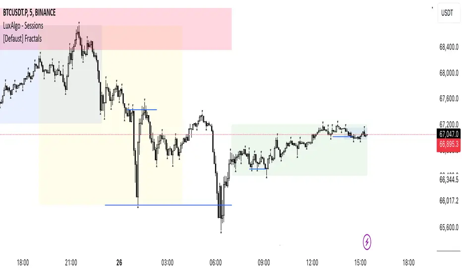
[Defaust] Fractals Fractals Indicator
Overview
The Fractals Indicator is a technical analysis tool designed to help traders identify potential reversal points in the market by detecting fractal patterns. This indicator is a fork of the original fractals indicator, with adjustments made to the plotting for enhanced visual clarity and usability.
What Are Fractals?
In trading, a fractal is a pattern consisting of five consecutive bars (candlesticks) that meet specific conditions:
Up Fractal (Potential Sell Signal): Occurs when a high point is surrounded by two lower highs on each side.
Down Fractal (Potential Buy Signal): Occurs when a low point is surrounded by two higher lows on each side.
Fractals help traders identify potential tops and bottoms in the market, signaling possible entry or exit points.
Features of the Indicator
Customizable Periods (n): Allows you to define the number of periods to consider when detecting fractals, offering flexibility to adapt to different trading strategies and timeframes.
Enhanced Plotting Adjustments: This fork introduces adjustments to the plotting of fractal signals for better visual representation on the chart.
Visual Signals: Plots up and down triangles on the chart to signify down fractals (potential bullish signals) and up fractals (potential bearish signals), respectively.
Overlay on Chart: The fractal signals are overlaid directly on the price chart for immediate visualization.
Adjustable Precision: You can set the precision of the plotted values according to your needs.
Pine Script Code Explanation
Below is the Pine Script code for the Fractals Indicator:
//@version=5 indicator(" Fractals", shorttitle=" Fractals", format=format.price, precision=0, overlay=true)
// User input for the number of periods to consider for fractal detection n = input.int(title="Periods", defval=2, minval=2)
// Initialize flags for up fractal detection bool upflagDownFrontier = true bool upflagUpFrontier0 = true bool upflagUpFrontier1 = true bool upflagUpFrontier2 = true bool upflagUpFrontier3 = true bool upflagUpFrontier4 = true
// Loop through previous and future bars to check conditions for up fractals for i = 1 to n // Check if the highs of previous bars are less than the current bar's high upflagDownFrontier := upflagDownFrontier and (high < high ) // Check various conditions for future bars upflagUpFrontier0 := upflagUpFrontier0 and (high < high ) upflagUpFrontier1 := upflagUpFrontier1 and (high <= high and high < high ) upflagUpFrontier2 := upflagUpFrontier2 and (high <= high and high <= high and high < high ) upflagUpFrontier3 := upflagUpFrontier3 and (high <= high and high <= high and high <= high and high < high ) upflagUpFrontier4 := upflagUpFrontier4 and (high <= high and high <= high and high <= high and high <= high and high < high )
// Combine the flags to determine if an up fractal exists flagUpFrontier = upflagUpFrontier0 or upflagUpFrontier1 or upflagUpFrontier2 or upflagUpFrontier3 or upflagUpFrontier4 upFractal = (upflagDownFrontier and flagUpFrontier)
// Initialize flags for down fractal detection bool downflagDownFrontier = true bool downflagUpFrontier0 = true bool downflagUpFrontier1 = true bool downflagUpFrontier2 = true bool downflagUpFrontier3 = true bool downflagUpFrontier4 = true
// Loop through previous and future bars to check conditions for down fractals for i = 1 to n // Check if the lows of previous bars are greater than the current bar's low downflagDownFrontier := downflagDownFrontier and (low > low ) // Check various conditions for future bars downflagUpFrontier0 := downflagUpFrontier0 and (low > low ) downflagUpFrontier1 := downflagUpFrontier1 and (low >= low and low > low ) downflagUpFrontier2 := downflagUpFrontier2 and (low >= low and low >= low and low > low ) downflagUpFrontier3 := downflagUpFrontier3 and (low >= low and low >= low and low >= low and low > low ) downflagUpFrontier4 := downflagUpFrontier4 and (low >= low and low >= low and low >= low and low >= low and low > low )
// Combine the flags to determine if a down fractal exists flagDownFrontier = downflagUpFrontier0 or downflagUpFrontier1 or downflagUpFrontier2 or downflagUpFrontier3 or downflagUpFrontier4 downFractal = (downflagDownFrontier and flagDownFrontier)
// Plot the fractal symbols on the chart with adjusted plotting plotshape(downFractal, style=shape.triangleup, location=location.belowbar, offset=-n, color=color.gray, size=size.auto) plotshape(upFractal, style=shape.triangledown, location=location.abovebar, offset=-n, color=color.gray, size=size.auto)
Explanation:
Input Parameter (n): Sets the number of periods for fractal detection. The default value is 2, and it must be at least 2 to ensure valid fractal patterns.
Flag Initialization: Boolean variables are used to store intermediate conditions during fractal detection.
Loops: Iterate through the specified number of periods to evaluate the conditions for fractal formation.
Conditions:
Up Fractals: Checks if the current high is greater than previous highs and if future highs are lower or equal to the current high.
Down Fractals: Checks if the current low is lower than previous lows and if future lows are higher or equal to the current low.
Flag Combination: Logical and and or operations are used to combine the flags and determine if a fractal exists.
Adjusted Plotting:
The plotting of fractal symbols has been adjusted for better alignment and visual clarity.
The offset parameter is set to -n to align the plotted symbols with the correct bars.
The color and size have been fine-tuned for better visibility.
How to Use the Indicator
Adding the Indicator to Your Chart
Open TradingView:
Go to TradingView.
Access the Chart:
Click on "Chart" to open the main charting interface.
Add the Indicator:
Click on the "Indicators" button at the top.
Search for " Fractals".
Select the indicator from the list to add it to your chart.
Configuring the Indicator
Periods (n):
Default value is 2.
Adjust this parameter based on your preferred timeframe and sensitivity.
A higher value of n considers more bars for fractal detection, potentially reducing the number of signals but increasing their significance.
Interpreting the Signals
– Up Fractal (Downward Triangle): Indicates a potential price reversal to the downside. May be used as a signal to consider exiting long positions or tightening stop-loss orders.
– Down Fractal (Upward Triangle): Indicates a potential price reversal to the upside. May be used as a signal to consider entering long positions or setting stop-loss orders for short positions.
Trading Strategy Suggestions
Up Fractal Detection:
The high of the current bar (n) is higher than the highs of the previous two bars (n - 1, n - 2).
The highs of the next bars meet certain conditions to confirm the fractal pattern.
An up fractal symbol (downward triangle) is plotted above the bar at position n - n (due to the offset).
Down Fractal Detection:
The low of the current bar (n) is lower than the lows of the previous two bars (n - 1, n - 2).
The lows of the next bars meet certain conditions to confirm the fractal pattern.
A down fractal symbol (upward triangle) is plotted below the bar at position n - n.
Benefits of Using the Fractals Indicator
Early Signals: Helps in identifying potential reversal points in price movements.
Customizable Sensitivity: Adjusting the n parameter allows you to fine-tune the indicator based on different market conditions.
Enhanced Visuals: Adjustments to plotting improve the clarity and readability of fractal signals on the chart.
Limitations and Considerations
Lagging Indicator: Fractals require future bars to confirm the pattern, which may introduce a delay in the signals.
False Signals: In volatile or ranging markets, fractals may produce false signals. It's advisable to use them in conjunction with other analysis tools.
Not a Standalone Tool: Fractals should be part of a broader trading strategy that includes other indicators and fundamental analysis.
Best Practices for Using This Indicator
Combine with Other Indicators: Use in combination with trend indicators, oscillators, or volume analysis to confirm signals.
Backtesting: Before applying the indicator in live trading, backtest it on historical data to understand its performance.
Adjust Periods Accordingly: Experiment with different values of n to find the optimal setting for the specific asset and timeframe you are trading.
Disclaimer
The Fractals Indicator is intended for educational and informational purposes only. Trading involves significant risk, and you should be aware of the risks involved before proceeding. Past performance is not indicative of future results. Always conduct your own analysis and consult with a professional financial advisor before making any investment decisions.
Credits
This indicator is a fork of the original fractals indicator, with adjustments made to the plotting for improved visual representation. It is based on standard fractal patterns commonly used in technical analysis and has been developed to provide traders with an effective tool for detecting potential reversal points in the market.
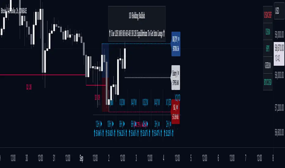
OptiRange | FractalystWhat’s the purpose of this indicator?
This indicator is designed to integrate probabilities with liquidity levels, while also providing a mechanical method for identifying market structure by using Fractals by Williams.
----
How does this indicator identify market structure?
This script identifies breaks of market structure by analyzing candle closures above or below swing levels.
As soon as a candle has closed above or below the initial swing on your charts, the script validates that there is at least one swing preceding the break before confirming it as a structural break.
Once a break is occured then it assigns a numeric ID to the break starting from 1 and draws two extremities: one as liquidity and the other as invalidation (LIQ/INV).
----
What do the extremities show us on the charts?
you'll see two clear extremities on your charts:
1. The first extremity represents the structural liquidity level. (LIQ)
2. The other extremity indicates the level that, if price breaks through it, results in a structural shift to the opposite side. (INV)
----
How does it calculate probabilities?
Each break of market structure, denoted as X, is assigned a unique ID, starting from X1 for the first break, X2 for the second, and so on.
The probabilities are calculated based on breaks holding, meaning price closing through the liquidity level, rather than invalidation. This probability is then divided by the total count of similar numeric breaks.
For example, if 75 out of 100 bullish X1s become X2, then the probability of X1 becoming X2 on your charts will be displayed as 80% in the following format: ⬆ 75%
----
What are the Fractal blocks?
Fractal blocks refer to the most extreme swing candle within the latest break. They can serve as significant levels for price rejection and may guide movements toward the next break, often in confluence with probability analysis for added confirmation.
If the price retraces back to a bullish fractal block, we aim to look for buy/long positions. Conversely, if the price retraces back to a bearish fractal block, we aim to look for sell/short positions.
----
What are mitigations?
Mitigations refer to specific price action occurrences identified by the script:
1- When the price reaches the most recent fractal block and confirms a swing candle, the script automatically draws a line from the swing to the fractal block bar and labels it with a checkmark.
1- If the price wicks through the invalidation level and then retraces back to the fractal block while forming a swing candle, the script labels this as a double mitigation on the chart.
This level will serve as the next potential invalidation level if a break occurs in the same direction.
----
What does the bottom table display?
The bottom table presents numeric breaks across multiple timeframes, with the text color indicating the trend direction. Enabling traders to assess the higher timeframes market trend without needing to switch between timeframes manually.
----
How to use the indicator?
1. Add "OptiRange | Fractalyst" to your TradingView chart.
2. Choose the pair you want to analyze or trade.
3. Start with the 12-month timeframe.
4. Use the table bias with the maximal settings to find the lowest timeframe that’s showing you the mitigation (✓)
5. Confirm that the probability of the current liquidity is higher than 50%.
6. Place your limit order at the Fibonacci level of 0.618 of the mitigation candle.
7. Set your stop-loss at the mitigation level.
8. Determine your take profit based on the liquidity of the current timeframe, or if possible, the liquidity of a higher timeframe in the same direction; otherwise, use the liquidity of the current timeframe.
9. Risk adjustment and Trade management based on your personal preferences.
Example:
----
User-input settings and customizations
----
What makes this indicator original?
- This script leverages Fractals, a fundamental concept in many trading methodologies.
- For a break to be considered valid, price must have at least two swings:
a swing high followed by a swing low for bullish breaks and a swing low follow by a swing high for bearish breaks.
- This means that each swing point is confirmed by the formation of two candles on its left and two candles on its right, totaling 5 candles for each swing high and swing low, thus requiring 10 candles overall. (This strict rule ensures a thorough assessment of market structure before confirming a break.)
- The script assigns a unique numerical ID to each break of structure, starting from 1.
This numbering system enables the script to calculate the probability of the most recent break becoming the next break, while also factoring in the trend direction.
- Additionally, this script provides insights into higher timeframes' break IDs in the bottom/top centre table, keeping traders informed about the overall higher timeframe picture.
- By integrating these methodologies, the script introduces a unique and systematic method for identifying market structure, thereby enhancing its originality in guiding trading decisions.
Terms and Conditions | Disclaimer
Our charting tools are provided for informational and educational purposes only and should not be construed as financial, investment, or trading advice. They are not intended to forecast market movements or offer specific recommendations. Users should understand that past performance does not guarantee future results and should not base financial decisions solely on historical data. By utilizing our charting tools, the buyer acknowledges that neither the seller nor the creator assumes responsibility for decisions made using the information provided. The buyer assumes full responsibility and liability for any actions taken and their consequences, including potential financial losses. Therefore, by purchasing these charting tools, the customer acknowledges that neither the seller nor the creator is liable for any unfavorable outcomes resulting from the development, sale, or use of the products.
The buyer is responsible for canceling their subscription if they no longer wish to continue at the full retail price. Our policy does not include reimbursement, refunds, or chargebacks once the Terms and Conditions are accepted before purchase.
By continuing to use our charting tools, the user acknowledges and accepts the Terms and Conditions outlined in this legal disclaimer.
Screener | FractalystWhat’s the purpose of this indicator?
This indicator is part of the Optirange suite , which analyzes all timeframes using a mechanical top-down approach to determine the overall market bias. It helps you identify the specific timeframes and exact levels for positioning in longs, shorts, or guiding you on whether to stay away from trading a particular market condition.
The purpose of the Screener indicator is to track the contextual bias of multiple markets simultaneously on the charts without the need to switch between pairs. This allows traders to monitor various assets in real-time, enhancing decision-making efficiency and identifying potential trading opportunities more effectively.
-----
How does this indicator identify the overall market bias?
This indicator employs a systematic top-down approach, analyzing market structure, fractal blocks, and their mitigations from the 12M timeframe down to the 1D timeframe to uncover the story behind the market. This method helps identify the overall market bias, whether it’s bullish, bearish, or in consolidating conditions.
Below is a flowchart that illustrates the calculation behind the market context identification, demonstrating the systematic approach:
-----
According to the above trade plan, why do we only look for mitigations within Fractal Blocks of X1/X2?
In this context, "X" stands for a break in the market's structure, and the numbers (1 and 2) indicate the sequence of these breaks within the same trend direction, either up or down.
We focus on mitigations within Fractal Blocks during the X1/X2 stages because these points mark the early phase (X1) and the continuation (X2) of a trend. By doing so, we align our trades with the market's main direction and avoid getting stopped out in the middle of trends.
-----
How does this indicator identify ranges in a mechanical way?
Since the indicator is part of the Optirange suite , it follows the exact rules that Optirange utilizes to identify breaks of market structures in a mechanical manner.
Let’s take a closer look at how the ranges are calculated:
1- First, we need to understand the importance of following a set of mechanical rules in identifying market structure:
The image above illustrates the difference between a subjective and a mechanical approach to analyzing market structure. The subjective method often leads to uncertainty, where traders might struggle to pinpoint exact breaks in structure, resulting in inconsistent decision-making. Questions like “Is this a break?” or “Maybe this one...?” reflect the ambiguity of manual interpretation, which can cause confusion and errors in trading.
On the other hand, the mechanical approach depicted on the right side of the image follows a clear, rule-based method to define breaks in market structure. This systematic approach eliminates guesswork by providing precise criteria for identifying structural changes, such as marking structural invalidation levels where market bias shifts from bullish to bearish or vice versa. The mechanical method not only offers consistency but also integrates statistical probabilities , enhancing the trader's ability to make data-driven decisions.
By adhering to these mechanical rules, the Screener indicator ensures that ranges are identified consistently, allowing traders to rely on objective analysis rather than subjective interpretation . This approach is crucial for accurately defining market structures and making informed trading decisions.
2- Now let's take a look at a practical example of how the indicator utilizes Pivot points with a period of 2 to identify ranges:
In this image, we see a Bearish Scenario on the left and a Bullish Scenario on the right. The indicator starts by identifying the first significant swing on the chart. It then validates this swing by checking if there is a preceding swing high (for a bearish scenario) or swing low (for a bullish scenario). Once validated, the indicator confirms a break of structure when price closes below or above these points, respectively.
For instance, in the Bearish Scenario:
The first significant swing is identified.
The script checks for a preceding swing high before confirming any structural break.
A candle closure below the swing low confirms the first bearish break of structure.
This results in a confirmed market bias towards bearishness, with structural liquidity levels indicated for potential price targets.
In the Bullish Scenario:
The process is mirrored, identifying the first swing low and validating it with a preceding swing low.
A closure above this swing confirms the bullish break of structure.
This leads to a market bias towards bullishness, with invalidation levels to watch if the trend shifts.
This practical example demonstrates how the indicator systematically identifies market ranges, ensuring that traders can make informed decisions based on clear, rule-based criteria.
-----
How does this indicator identify ranges in a mechanical way, What are the underlying calculations?
Fractal blocks refer to the most extreme swing candle within the latest break. They can serve as significant levels for price rejection and may guide movements toward the next break, often in confluence with topdown analysis for added confirmation.
-----
What are mitigations, What are the underlying calculations?
Mitigations refer to specific price action occurrences identified by the script:
1- When the price reaches the most recent fractal block and confirms a swing candle, the script automatically draws a line from the swing to the fractal block bar and labels it with a checkmark.
2- If the price wicks through the invalidation level and then retraces back to the fractal block while forming a swing candle, the script labels this as a double mitigation on the chart.
This level will serve as the next potential invalidation level if a break occurs in the same direction.
-----
What does the right table display?
The table located at the right of your chart displays five colored symbols that represent the contextual market bias:
Green: The market is in a bullish condition.
Red: The market is in a bearish condition.
White: The market condition is uncertain, and it is advisable to stay away from trading.
-----
What does the bottom table display?
The bottom table can be turned on in the Optirange indicator and serves multiple purposes:
Range Counts and Mitigations: It shows the range counts and their mitigations across multiple timeframes, providing a comprehensive view of market dynamics.
Hourly Timeframe Probabilities: The bottom row of the bias table displays the probabilities for various hourly timeframes, helping to identify potential entry levels based on the multi-timeframe bias determined by the Screener.
In a bullish market context, you should look for long positions by focusing on hourly timeframes where buy-side probability exceeds 50%.
In a bearish market context, you should look for short positions by focusing on hourly timeframes where the sell-side probability exceeds 50%.
When the symbol is white within the Screener table, it signals that the market bias is unclear, and it's recommended to stay away from trading in such conditions.
-----
How the range probabilities are calculated?
Each break of market structure, denoted as X, is assigned a unique ID, starting from X1 for the first break, X2 for the second, and so on.
The probabilities are calculated based on breaks holding, meaning price closing through the liquidity level, rather than invalidation. This probability is then divided by the total count of similar numeric breaks.
For example, if 75 out of 100 bullish X1s become X2, then the probability of X1 becoming X2 on your charts will be displayed as 75% in the following format: ⬆ 75%
-----
What does the top table display?
The top table on the charts displays the current market context, offering insights into the underlying bias. It highlights the high-timeframe (HTF) bias and guides you on which timeframes you should use to enter long or short positions, based on the probability of success.
Additionally, when the market bias is unclear, the table clearly signals that it's best to avoid trading that specific market until the context or market story becomes clearer. This helps traders make informed decisions and avoid uncertain market conditions.
-----
How does the Screener indicator identify the market bias/context/story ?
- Market Structure: The Optirange indicator analyzes market structure across multiple timeframes, from a top-down perspective, including 12M, 6M, 3M, 1M, 2W, 1W, 3D, and 1D.
- Fractal Blocks: Once the market structure or current range is identified, the indicator automatically identifies the last push before the break and draws it as a box. These zones acts as a key area where the price often rejects from.
- Mitigations: After identifying the Fractal Block, the indicator checks for price mitigation or rejection within this zone. If mitigation occurs, meaning the price has reacted or rejected from the Fractal Block, the indicator draws a checkmark from the deepest candle within the Fractal Block to the initial candle that has created the zone.
- Bias Table: After identifying the three key elements—market structure, Fractal Blocks, and price mitigations—the indicator compiles this information into a multi-timeframe table. This table provides a comprehensive top-down perspective, showing what is happening from a structural standpoint across all timeframes. The Bias Table presents raw data, including identified Fractal Blocks and mitigations, to help traders understand the overall market trend. This data is crucial for the screener, which uses it to determine the current market bias based on a top-down analysis.
- Screener: Once all higher timeframes (HTF) and lower timeframes (LTF) are calculated using the indicator, it follows the exact rules outlined in the flowchart to determine the market bias. This systematic approach not only helps identify the current market trend but also suggests the exact timeframes to use for finding entry, particularly on hourly timeframes.
Example:
12M Timeframe:
OANDA:EURUSD
6M Timeframe :
OANDA:EURUSD
3M Timeframe :
OANDA:EURUSD
1M Timeframe :
OANDA:EURUSD
2W Timeframe :
OANDA:EURUSD
1W Timeframe :
OANDA:EURUSD
-----
User-input settings and customizations
Terms and Conditions | Disclaimer
Our charting tools are provided for informational and educational purposes only and should not be construed as financial, investment, or trading advice. They are not intended to forecast market movements or offer specific recommendations. Users should understand that past performance does not guarantee future results and should not base financial decisions solely on historical data. By utilizing our charting tools, the buyer acknowledges that neither the seller nor the creator assumes responsibility for decisions made using the information provided. The buyer assumes full responsibility and liability for any actions taken and their consequences, including potential financial losses. Therefore, by purchasing these charting tools, the customer acknowledges that neither the seller nor the creator is liable for any unfavorable outcomes resulting from the development, sale, or use of the products.
The buyer is responsible for canceling their subscription if they no longer wish to continue at the full retail price. Our policy does not include reimbursement, refunds, or chargebacks once the Terms and Conditions are accepted before purchase.
By continuing to use our charting tools, the user acknowledges and accepts the Terms and Conditions outlined in this legal disclaimer.
Whale Fractal Levels (V1.0)What it does
This indicator plots Fractal Levels (Bill Williams pivots) as horizontal lines and prints clean signals for:
BO+ / BO− → Breakouts through the latest fractal high/low
SW↑ / SW↓ → Liquidity sweeps (wick pierces, close rejects)
RE+ / RE− → Retests of the broken level after a confirmed breakout
Cyan = support (fractal lows).
Lilac = resistance (fractal highs).
How it works
Detects fractals with Left/Right = lr. A pivot is confirmed after lr bars on the right → the level itself doesn’t repaint.
Each confirmed fractal spawns a horizontal line extended to the right. You can limit how many lines stay on chart and auto-expire old ones.
Signals reference the most recent fractal high/low only and are edge-triggered (crossover/crossunder) with a cooldown so you don’t get a marker on every bar near the level.
A small state machine remembers the last breakout to validate the next retest.
Inputs (Settings)
Fractals
Left/Right (BW fractal) — Sensitivity of pivots (lower = more reactive, higher = cleaner).
MAX number of levels to display — Keep only the most recent N lines.
Level lifetime (bars) — Auto-delete lines after N bars to declutter.
Signals
Cooldown between signals (bars) — Minimum spacing between markers (anti-spam).
Show Breakouts (BO±) — Toggle breakout markers.
Show Sweeps (SW↑/SW↓) — Toggle sweep markers.
Show Retests (RE±) — Toggle retest markers.
Display
Show fractal lines / Line width / Line transparency (0..100)
Alerts (ready to use)
BO+ (Fractal), BO- (Fractal)
SW↑ (Fractal), SW↓ (Fractal)
RE+ (Fractal), RE- (Fractal)

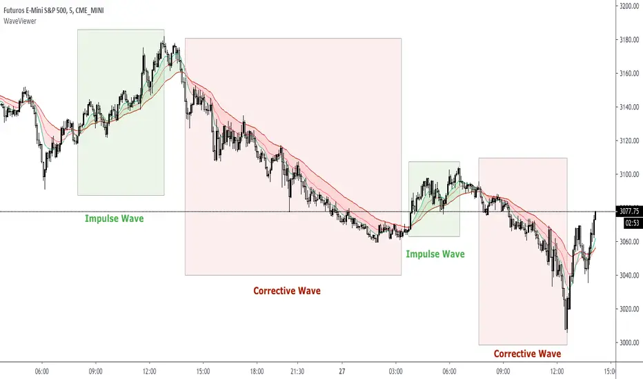
WaveViewer
WaveViewer impulsive and corrective wave viewer indicator
The market is developed by making impulsive wave movements and corrective waves thus forming a "V" type fractal
This indicator allows you to easily visualize these movements to make buying or selling decisions
WaveViewer is an indicator that allows the identification of impulsive waves visually through EMAs crossings
Visually facilitates the green color for the impulsive wave and red for the corrective wave
NOTE 1: This indicator should be complemented with the 1-9 fractal counter
NOTE 2: WaveViewer recommended for instrument ES1 ( SP500 ) with timeframe 5 minutes
Hidden Markov Model [Extension] | FractalystWhat's the indicator's purpose and functionality?
The Hidden Markov Model is specifically designed to integrate with the Quantify Trading Model framework, serving as a probabilistic market regime identification system for institutional trading analysis.
Hidden Markov Models are particularly well-suited for market regime detection because they can model the unobservable (hidden) state of the market, capture probabilistic transitions between different states, and account for observable market data that each state generates.
The indicator uses Hidden Markov Model mathematics to automatically detect distinct market regimes such as low-volatility bull markets, high-volatility bear markets, or range-bound consolidation periods.
This approach provides real-time regime probabilities without requiring optimization periods that can lead to overfitting, enabling systematic trading based on genuine probabilistic market structure.
How does this extension work with the Quantify Trading Model?
The Hidden Markov Model | Fractalyst serves as a probabilistic state estimation engine for systematic market analysis.
Instead of relying on traditional technical indicators, this system automatically identifies market regimes using forward algorithm implementation with three-state probability calculation (bullish/neutral/bearish), Viterbi decoding process for determining most likely regime sequence without repainting, online parameter learning with adaptive emission probabilities based on market observations, and multi-feature analysis combining normalized returns, volatility comprehensive regime assessment.
The indicator outputs regime probabilities and confidence levels that can be used for systematic trading decisions, portfolio allocation, or risk management protocols.
Why doesn't this use optimization periods like other indicators?
The Hidden Markov Model | Fractalyst deliberately avoids optimization periods to prevent overfitting bias that destroys out-of-sample performance.
The system uses a fixed mathematical framework based on Hidden Markov Model theory rather than optimized parameters, probabilistic state estimation using forward algorithm calculations that work across all market conditions, online learning methodology with adaptive parameter updates based on real-time market observations, and regime persistence modeling using fixed transition probabilities with 70% diagonal bias for realistic regime behavior.
This approach ensures the regime detection signals remain robust across different market cycles without the performance degradation typical of over-optimized traditional indicators.
Can this extension be used independently for discretionary trading?
No, the Hidden Markov Model | Fractalyst is specifically engineered for systematic implementation within institutional trading frameworks.
The indicator is designed to provide regime filtering for systematic trading algorithms and risk management systems, enable automated backtesting through mathematical regime identification without subjective interpretation, and support institutional-level analysis when combined with systematic entry/exit models.
Using this indicator independently would miss the primary value proposition of systematic regime-based strategy optimization that institutional frameworks provide.
How do I integrate this with the Quantify Trading Model?
Integration enables institutional-grade systematic trading through advanced machine learning and statistical validation:
- Add both HMM Extension and Quantify Trading Model to your chart
- Select HMM Extension as the bias source using input.source()
- Quantify automatically uses the extension's bias signals for entry/exit analysis
- The built-in machine learning algorithms score optimal entry and exit levels based on trend intensity, and market structure patterns identified by the extension
The extension handles all bias detection complexity while Quantify focuses on optimal trade timing, position sizing, and risk management along with PineConnector automation
What markets and assets does the indicator Extension work best on?
The Hidden Markov Model | Fractalyst performs optimally on markets with sufficient price movement since the system relies on statistical analysis of returns, volatility, and momentum patterns for regime identification.
Recommended asset classes include major forex pairs (EURUSD, GBPUSD, USDJPY) with high liquidity and clear regime transitions, stock index futures (ES, NQ, YM) providing consistent regime behavior patterns, individual equities (large-cap stocks with sufficient volatility for regime detection), cryptocurrency markets (BTC, ETH with pronounced regime characteristics), and commodity futures (GC, CL showing distinct market cycles and regime transitions).
These markets provide sufficient statistical variation in returns and volatility patterns, ensuring the HMM system's mathematical framework can effectively distinguish between bullish, neutral, and bearish regime states.
Any timeframe from 15-minute to daily charts provides sufficient data points for regime calculation, with higher timeframes (4H, Daily) typically showing more stable regime identification with fewer false transitions, while lower timeframes (30m, 1H) provide more responsive regime detection but may show increased noise.
Acceptable Timeframes and Portfolio Integration:
- Any timeframe that can be evaluated within Quantify Trading Model's backtesting engine is acceptable for live trading implementation.
Legal Disclaimers and Risk Acknowledgments
Trading Risk Disclosure
The HMM Extension is provided for informational, educational, and systematic bias detection purposes only and should not be construed as financial, investment, or trading advice. The extension provides institutional analysis but does not guarantee profitable outcomes, accurate bias predictions, or positive investment returns.
Trading systems utilizing bias detection algorithms carry substantial risks including but not limited to total capital loss, incorrect bias identification, market regime changes, and adverse conditions that may invalidate analysis. The extension's performance depends on accurate data, TradingView infrastructure stability, and proper integration with Quantify Trading Model, any of which may experience data errors, technical failures, or service interruptions that could affect bias detection accuracy.
System Dependency Acknowledgment
The extension requires continuous operation of multiple interconnected systems: TradingView charts and real-time data feeds, accurate reporting from exchanges, Quantify Trading Model integration, and stable platform connectivity. Any interruption or malfunction in these systems may result in incorrect bias signals, missed transitions, or unexpected analytical behavior.
Users acknowledge that neither Fractalyst nor the creator has control over third-party data providers, exchange reporting accuracy, or TradingView platform stability, and cannot guarantee data accuracy, service availability, or analytical performance. Market microstructure changes, reporting delays, exchange outages, and technical factors may significantly affect bias detection accuracy compared to theoretical or backtested performance.
Intellectual Property Protection
The HMM Extension, including all proprietary algorithms, classification methodologies, three-state bias detection systems, and integration protocols, constitutes the exclusive intellectual property of Fractalyst. Unauthorized reproduction, reverse engineering, modification, or commercial exploitation of these proprietary technologies is strictly prohibited and may result in legal action.
Liability Limitation
By utilizing this extension, users acknowledge and agree that they assume full responsibility and liability for all trading decisions, financial outcomes, and potential losses resulting from reliance on the extension's bias detection signals. Fractalyst shall not be liable for any unfavorable outcomes, financial losses, missed opportunities, or damages resulting from the development, use, malfunction, or performance of this extension.
Past performance of bias detection accuracy, classification effectiveness, or integration with Quantify Trading Model does not guarantee future results. Trading outcomes depend on numerous factors including market regime changes, pattern evolution, institutional behavior shifts, and proper system configuration, all of which are beyond the control of Fractalyst.
User Responsibility Statement
Users are solely responsible for understanding the risks associated with algorithmic bias detection, properly configuring system parameters, maintaining appropriate risk management protocols, and regularly monitoring extension performance. Users should thoroughly validate the extension's bias signals through comprehensive backtesting before live implementation and should never base trading decisions solely on automated bias detection.
This extension is designed to provide systematic institutional flow analysis but does not replace the need for proper market understanding, risk management discipline, and comprehensive trading methodology. Users should maintain active oversight of bias detection accuracy and be prepared to implement manual overrides when market conditions invalidate analysis assumptions.
Terms of Service Acceptance
Continued use of the HMM Extension constitutes acceptance of these terms, acknowledgment of associated risks, and agreement to respect all intellectual property protections. Users assume full responsibility for compliance with applicable laws and regulations governing automated trading system usage in their jurisdiction.

VWAP/VOL [Extension] | FractalystWhat's the indicator's purpose and functionality?
The VWAP/VOL Extension is designed specifically as a bias identification system for the Quantify Trading Model.
This extension uses volume-weighted average price analysis combined with institutional volume classification to automatically detect market bias without requiring optimization periods that lead to overfitting.
The system provides real-time bias signals (bullish/bearish/neutral) that integrate directly with Quantify's machine learning algorithms, enabling institutional-level backtesting and automated entry/exit identification based on genuine market structure rather than curve-fitted parameters.
How does this extension work with the Quantify Trading Model?
The VWAP/VOL Extension serves as the bias detection engine for Quantify's automated trading system.
Instead of manually selecting bias direction, this extension automatically identifies market bias using:
- Volume-weighted VWAP analysis with three-state detection (bullish/bearish/neutral)
- Institutional volume classification using relative volume thresholds without optimization
- Non-repainting architecture ensuring consistent bias signals for Quantify's machine learning
The extension outputs bias signals that Quantify uses as input through the `input.source()` function, allowing the Trading Model to focus on optimal entry/exit timing while the extension handles bias identification.
Why doesn't this use optimization periods like other indicators?
The VWAP/VOL Extension deliberately avoids optimization periods to prevent overfitting bias that destroys out-of-sample performance. The system uses:
- Fixed mathematical thresholds based on market structure principles rather than optimized parameters
- Relative volume analysis using standard 2.0x/0.5x ratios that work across all market conditions
- VWAP distance calculations based on percentage thresholds without curve-fitting
- Gap enforcement using fixed 5-bar minimums for disciplined bias detection
This approach ensures the bias signals remain robust across different market regimes without the performance degradation typical of over-optimized systems.
Can this extension be used independently for discretionary trading?
No, the VWAP/VOL Extension is specifically engineered to work as a component within the Quantify ecosystem. The extension is designed to:
- Provide bias input for Quantify's machine learning algorithms
- Enable automated backtesting through systematic bias identification
- Support institutional-level analysis when combined with Quantify's ML entry model
Using this extension independently would miss the primary value proposition of systematic entry/exit optimization that Quantify provides.
The extension handles bias detection so Quantify can focus on probability-based trade timing and risk management.
How does this enable institutional-level backtesting?
The extension transforms discretionary bias identification into systematic institutional analysis by:
- Eliminating subjective bias selection through automated VWAP/volume analysis
- Providing consistent historical signals with non-repainting architecture for accurate backtesting
- Integrating with Quantify's algorithms to identify optimal entry patterns based on objective bias states
- Enabling performance analysis across multiple market regimes without optimization bias
This combination allows Quantify to run institutional-grade backtests with consistent bias identification, generating reliable performance statistics and risk metrics that reflect genuine market edge rather than curve-fitted results.
How do I integrate this with the Quantify Trading Model?
Integration enables institutional-grade systematic trading through advanced machine learning and statistical validation:
- Add both VWAP/VOL Extension and Quantify Trading Model to your chart
- Select VWAP/VOL Extension as the bias source using input.source()
- Quantify automatically uses the extension's bias signals for entry/exit analysis
- The built-in machine learning algorithms score optimal entry and exit levels based on trend intensity, volume conviction, and market structure patterns identified by the extension
The extension handles all bias detection complexity while Quantify focuses on optimal trade timing, position sizing, and risk management along with PineConnector automation
What markets and assets does the VWAP/VOL Extension work best on?
The VWAP/VOL Extension performs optimally on markets with consistent, high-volume participation since the system relies on institutional volume analysis for bias detection. Futures markets provide the most reliable performance due to their centralized volume data and continuous institutional participation.
Recommended Futures Markets:
- ES (S&P 500 E-mini) - Over 2 million contracts daily volume, excellent liquidity depth
- NQ (NASDAQ-100 E-mini) - Around 600,000 contracts daily, strong tech sector representation
- YM (Dow Jones E-mini) - Consistent institutional flow and volume patterns
- RTY (Russell 2000 E-mini) - Small-cap exposure with reliable volume data
- GC (Gold Futures) - High volume commodity with institutional participation
- CL (Crude Oil Futures) - Energy sector representation with strong volume consistency
Why Futures Markets Excel:
- Futures markets provide centralized volume reporting, ensuring the extension's volume classification system receives accurate institutional participation data. The standardized contract specifications and continuous trading hours create consistent volume patterns that the extension's algorithms can analyze effectively.
Acceptable Timeframes and Portfolio Integration:
- Any timeframe that can be evaluated within Quantify Trading Model's backtesting engine is acceptable for live trading implementation.
The extension is specifically designed to integrate with Quantify's portfolio management system, allowing multiple strategies across different timeframes and assets to operate simultaneously while maintaining consistent bias identification methodology across the entire automated trading portfolio.
Legal Disclaimers and Risk Acknowledgments
Trading Risk Disclosure
The VWAP/VOL Extension is provided for informational, educational, and systematic bias detection purposes only and should not be construed as financial, investment, or trading advice. The extension provides volume-weighted institutional analysis but does not guarantee profitable outcomes, accurate bias predictions, or positive investment returns.
Trading systems utilizing bias detection algorithms carry substantial risks including but not limited to total capital loss, incorrect bias identification, market regime changes, and adverse conditions that may invalidate volume-based analysis. The extension's performance depends on accurate volume data, TradingView infrastructure stability, and proper integration with Quantify Trading Model, any of which may experience data errors, technical failures, or service interruptions that could affect bias detection accuracy.
System Dependency Acknowledgment
The extension requires continuous operation of multiple interconnected systems: TradingView charts and real-time data feeds, accurate volume reporting from exchanges, Quantify Trading Model integration, and stable platform connectivity. Any interruption or malfunction in these systems may result in incorrect bias signals, missed transitions, or unexpected analytical behavior.
Users acknowledge that neither Fractalyst nor the creator has control over third-party data providers, exchange volume reporting accuracy, or TradingView platform stability, and cannot guarantee data accuracy, service availability, or analytical performance. Market microstructure changes, volume reporting delays, exchange outages, and technical factors may significantly affect bias detection accuracy compared to theoretical or backtested performance.
Intellectual Property Protection
The VWAP/VOL Extension, including all proprietary algorithms, volume classification methodologies, three-state bias detection systems, and integration protocols, constitutes the exclusive intellectual property of Fractalyst. Unauthorized reproduction, reverse engineering, modification, or commercial exploitation of these proprietary technologies is strictly prohibited and may result in legal action.
Liability Limitation
By utilizing this extension, users acknowledge and agree that they assume full responsibility and liability for all trading decisions, financial outcomes, and potential losses resulting from reliance on the extension's bias detection signals. Fractalyst shall not be liable for any unfavorable outcomes, financial losses, missed opportunities, or damages resulting from the development, use, malfunction, or performance of this extension.
Past performance of bias detection accuracy, volume classification effectiveness, or integration with Quantify Trading Model does not guarantee future results. Trading outcomes depend on numerous factors including market regime changes, volume pattern evolution, institutional behavior shifts, and proper system configuration, all of which are beyond the control of Fractalyst.
User Responsibility Statement
Users are solely responsible for understanding the risks associated with algorithmic bias detection, properly configuring system parameters, maintaining appropriate risk management protocols, and regularly monitoring extension performance. Users should thoroughly validate the extension's bias signals through comprehensive backtesting before live implementation and should never base trading decisions solely on automated bias detection.
This extension is designed to provide systematic institutional flow analysis but does not replace the need for proper market understanding, risk management discipline, and comprehensive trading methodology. Users should maintain active oversight of bias detection accuracy and be prepared to implement manual overrides when market conditions invalidate volume-based analysis assumptions.
Terms of Service Acceptance
Continued use of the VWAP/VOL Extension constitutes acceptance of these terms, acknowledgment of associated risks, and agreement to respect all intellectual property protections. Users assume full responsibility for compliance with applicable laws and regulations governing automated trading system usage in their jurisdiction.

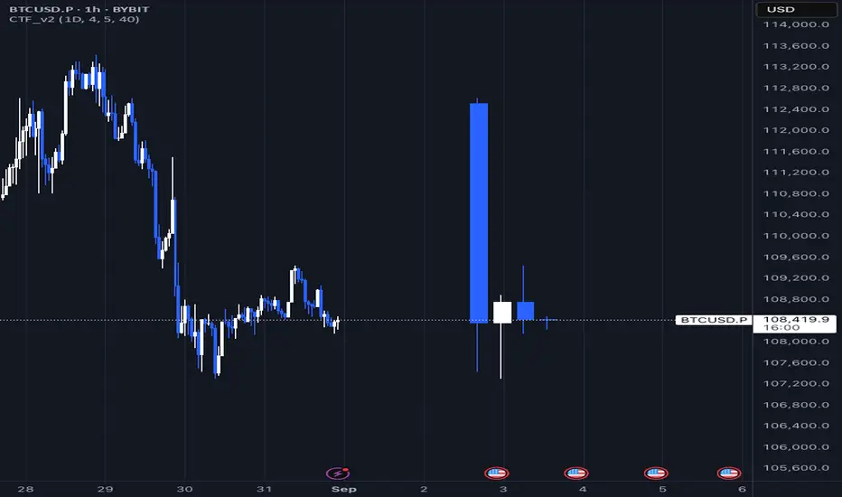
Daily Fractals Custom Timeframe Candles - Fractal Analysis Tool
📊 Overview
Custom Timeframe Candles is a powerful Pine Script indicator that displays higher timeframe (HTF) candles directly on your current chart, enabling seamless fractal analysis without switching between timeframes.
Perfect for traders who want to analyze daily candles while trading on hourly charts, or any other timeframe combination.
✨ Key Features
🎯 Multi-Timeframe Analysis
- Display any higher timeframe candles on your current chart
- Real-time updates of the current HTF candle as price moves
- Configurable number of candles (1-10) to display
🎮 How to Use
1. Add to Chart : Apply the indicator to any timeframe chart
2. Select HTF : Choose your desired higher timeframe (e.g., "1D" for daily)
3. Configure Display : Set number of candles, colors, and position
4. Analyze : View HTF context while trading on lower timeframes
📈 Perfect For Backtest
Unlike basic HTF displays, this indicator provides:
- Live Updates: Current candle updates in real-time
- Complete OHLC: Full candle structure with wicks
- Flexible Count: Display exactly what you need
- Stable Performance: No crashes during replay/backtesting
- Professional Design: Clean, customizable appearance
📝 Notes
- Works on all timeframes and instruments
- Requires higher timeframe data availability
- Compatible with replay mode and backtesting
---
by Rock9808
Williams Fractals with alerts ABCAll the original Williams Fractals algorithm but with a useful way to set up alerts.

PnL Bubble [%] | Fractalyst1. What's the indicator purpose?
The PnL Bubble indicator transforms your strategy's trade PnL percentages into an interactive bubble chart with professional-grade statistics and performance analytics. It helps traders quickly assess system profitability, understand win/loss distribution patterns, identify outliers, and make data-driven strategy improvements.
How does it work?
Think of this indicator as a visual report card for your trading performance. Here's what it does:
What You See
Colorful Bubbles: Each bubble represents one of your trades
Blue/Cyan bubbles = Winning trades (you made money)
Red bubbles = Losing trades (you lost money)
Bigger bubbles = Bigger wins or losses
Smaller bubbles = Smaller wins or losses
How It Organizes Your Trades:
Like a Photo Album: Instead of showing all your trades at once (which would be messy), it shows them in "pages" of 500 trades each:
Page 1: Your first 500 trades
Page 2: Trades 501-1000
Page 3: Trades 1001-1500, etc.
What the Numbers Tell You:
Average Win: How much money you typically make on winning trades
Average Loss: How much money you typically lose on losing trades
Expected Value (EV): Whether your trading system makes money over time
Positive EV = Your system is profitable long-term
Negative EV = Your system loses money long-term
Payoff Ratio (R): How your average win compares to your average loss
R > 1 = Your wins are bigger than your losses
R < 1 = Your losses are bigger than your wins
Why This Matters:
At a Glance: You can instantly see if you're a profitable trader or not
Pattern Recognition: Spot if you have more big wins than big losses
Performance Tracking: Watch how your trading improves over time
Realistic Expectations: Understand what "average" performance looks like for your system
The Cool Visual Effects:
Animation: The bubbles glow and shimmer to make the chart more engaging
Highlighting: Your biggest wins and losses get extra attention with special effects
Tooltips: hover any bubble to see details about that specific trade.
What are the underlying calculations?
The indicator processes trade PnL data using a dual-matrix architecture for optimal performance:
Dual-Matrix System:
• Display Matrix (display_matrix): Bounded to 500 trades for rendering performance
• Statistics Matrix (stats_matrix): Unbounded storage for complete statistical accuracy
Trade Classification & Aggregation:
// Separate wins, losses, and break-even trades
if val > 0.0
pos_sum += val // Sum winning trades
pos_count += 1 // Count winning trades
else if val < 0.0
neg_sum += val // Sum losing trades
neg_count += 1 // Count losing trades
else
zero_count += 1 // Count break-even trades
Statistical Averages:
avg_win = pos_count > 0 ? pos_sum / pos_count : na
avg_loss = neg_count > 0 ? math.abs(neg_sum) / neg_count : na
Win/Loss Rates:
total_obs = pos_count + neg_count + zero_count
win_rate = pos_count / total_obs
loss_rate = neg_count / total_obs
Expected Value (EV):
ev_value = (avg_win × win_rate) - (avg_loss × loss_rate)
Payoff Ratio (R):
R = avg_win ÷ |avg_loss|
Contribution Analysis:
ev_pos_contrib = avg_win × win_rate // Positive EV contribution
ev_neg_contrib = avg_loss × loss_rate // Negative EV contribution
How to integrate with any trading strategy?
Equity Change Tracking Method:
//@version=6
strategy("Your Strategy with Equity Change Export", overlay=true)
float prev_trade_equity = na
float equity_change_pct = na
if barstate.isconfirmed and na(prev_trade_equity)
prev_trade_equity := strategy.equity
trade_just_closed = strategy.closedtrades != strategy.closedtrades
if trade_just_closed and not na(prev_trade_equity)
current_equity = strategy.equity
equity_change_pct := ((current_equity - prev_trade_equity) / prev_trade_equity) * 100
prev_trade_equity := current_equity
else
equity_change_pct := na
plot(equity_change_pct, "Equity Change %", display=display.data_window)
Integration Steps:
1. Add equity tracking code to your strategy
2. Load both strategy and PnL Bubble indicator on the same chart
3. In bubble indicator settings, select your strategy's equity tracking output as data source
4. Configure visualization preferences (colors, effects, page navigation)
How does the pagination system work?
The indicator uses an intelligent pagination system to handle large trade datasets efficiently:
Page Organization:
• Page 1: Trades 1-500 (most recent)
• Page 2: Trades 501-1000
• Page 3: Trades 1001-1500
• Page N: Trades to
Example: With 1,500 trades total (3 pages available):
• User selects Page 1: Shows trades 1-500
• User selects Page 4: Automatically falls back to Page 3 (trades 1001-1500)
5. Understanding the Visual Elements
Bubble Visualization:
• Color Coding: Cyan/blue gradients for wins, red gradients for losses
• Size Mapping: Bubble size proportional to trade magnitude (larger = bigger P&L)
• Priority Rendering: Largest trades displayed first to ensure visibility
• Gradient Effects: Color intensity increases with trade magnitude within each category
Interactive Tooltips:
Each bubble displays quantitative trade information:
tooltip_text = outcome + " | PnL: " + pnl_str +
"\nDate: " + date_str + " " + time_str +
"\nTrade #" + str.tostring(trade_number) + " (Page " + str.tostring(active_page) + ")" +
"\nRank: " + str.tostring(rank) + " of " + str.tostring(n_display_rows) +
"\nPercentile: " + str.tostring(percentile, "#.#") + "%" +
"\nMagnitude: " + str.tostring(magnitude_pct, "#.#") + "%"
Example Tooltip:
Win | PnL: +2.45%
Date: 2024.03.15 14:30
Trade #1,247 (Page 3)
Rank: 5 of 347
Percentile: 98.6%
Magnitude: 85.2%
Reference Lines & Statistics:
• Average Win Line: Horizontal reference showing typical winning trade size
• Average Loss Line: Horizontal reference showing typical losing trade size
• Zero Line: Threshold separating wins from losses
• Statistical Labels: EV, R-Ratio, and contribution analysis displayed on chart
What do the statistical metrics mean?
Expected Value (EV):
Represents the mathematical expectation per trade in percentage terms
EV = (Average Win × Win Rate) - (Average Loss × Loss Rate)
Interpretation:
• EV > 0: Profitable system with positive mathematical expectation
• EV = 0: Break-even system, profitability depends on execution
• EV < 0: Unprofitable system with negative mathematical expectation
Example: EV = +0.34% means you expect +0.34% profit per trade on average
Payoff Ratio (R):
Quantifies the risk-reward relationship of your trading system
R = Average Win ÷ |Average Loss|
Interpretation:
• R > 1.0: Wins are larger than losses on average (favorable risk-reward)
• R = 1.0: Wins and losses are equal in magnitude
• R < 1.0: Losses are larger than wins on average (unfavorable risk-reward)
Example: R = 1.5 means your average win is 50% larger than your average loss
Contribution Analysis (Σ):
Breaks down the components of expected value
Positive Contribution (Σ+) = Average Win × Win Rate
Negative Contribution (Σ-) = Average Loss × Loss Rate
Purpose:
• Shows how much wins contribute to overall expectancy
• Shows how much losses detract from overall expectancy
• Net EV = Σ+ - Σ- (Expected Value per trade)
Example: Σ+: 1.23% means wins contribute +1.23% to expectancy
Example: Σ-: -0.89% means losses drag expectancy by -0.89%
Win/Loss Rates:
Win Rate = Count(Wins) ÷ Total Trades
Loss Rate = Count(Losses) ÷ Total Trades
Shows the probability of winning vs losing trades
Higher win rates don't guarantee profitability if average losses exceed average wins
7. Demo Mode & Synthetic Data Generation
When using built-in sources (close, open, etc.), the indicator generates realistic demo trades for testing:
if isBuiltInSource(source_data)
// Generate random trade outcomes with realistic distribution
u_sign = prand(float(time), float(bar_index))
if u_sign < 0.5
v_push := -1.0 // Loss trade
else
// Skewed distribution favoring smaller wins (realistic)
u_mag = prand(float(time) + 9876.543, float(bar_index) + 321.0)
k = 8.0 // Skewness factor
t = math.pow(u_mag, k)
v_push := 2.5 + t * 8.0 // Win trade
Demo Characteristics:
• Realistic win/loss distribution mimicking actual trading patterns
• Skewed distribution favoring smaller wins over large wins
• Deterministic randomness for consistent demo results
• Includes jitter effects to prevent visual overlap
8. Performance Limitations & Optimizations
Display Constraints:
points_count = 500 // Maximum 500 dots per page for optimal performance
Pine Script v6 Limits:
• Label Count: Maximum 500 labels per indicator
• Line Count: Maximum 100 lines per indicator
• Box Count: Maximum 50 boxes per indicator
• Matrix Size: Efficient memory management with dual-matrix system
Optimization Strategies:
• Pagination System: Handle unlimited trades through 500-trade pages
• Priority Rendering: Largest trades displayed first for maximum visibility
• Dual-Matrix Architecture: Separate display (bounded) from statistics (unbounded)
• Smart Fallback: Automatic page clamping prevents empty displays
Impact & Workarounds:
• Visual Limitation: Only 500 trades visible per page
• Statistical Accuracy: Complete dataset used for all calculations
• Navigation: Use page input to browse through entire trade history
• Performance: Smooth operation even with thousands of trades
9. Statistical Accuracy Guarantees
Data Integrity:
• Complete Dataset: Statistics matrix stores ALL trades without limit
• Proper Aggregation: Separate tracking of wins, losses, and break-even trades
• Mathematical Precision: Pine Script v6's enhanced floating-point calculations
• Dual-Matrix System: Display limitations don't affect statistical accuracy
Calculation Validation:
// Verified formulas match standard trading mathematics
avg_win = pos_sum / pos_count // Standard average calculation
win_rate = pos_count / total_obs // Standard probability calculation
ev_value = (avg_win * win_rate) - (avg_loss * loss_rate) // Standard EV formula
Accuracy Features:
• Mathematical Correctness: Formulas follow established trading statistics
• Data Preservation: Complete dataset maintained for all calculations
• Precision Handling: Proper rounding and boundary condition management
• Real-Time Updates: Statistics recalculated on every new trade
10. Advanced Technical Features
Real-Time Animation Engine:
// Shimmer effects with sine wave modulation
offset = math.sin(shimmer_t + phase) * amp
// Dynamic transparency with organic flicker
new_transp = math.min(flicker_limit, math.max(-flicker_limit, cur_transp + dir * flicker_step))
• Sine Wave Shimmer: Dynamic glowing effects on bubbles
• Organic Flicker: Random transparency variations for natural feel
• Extreme Value Highlighting: Special visual treatment for outliers
• Smooth Animations: Tick-based updates for fluid motion
Magnitude-Based Priority Rendering:
// Sort trades by magnitude for optimal visual hierarchy
sort_indices_by_magnitude(values_mat)
• Largest First: Most important trades always visible
• Intelligent Sorting: Custom bubble sort algorithm for trade prioritization
• Performance Optimized: Efficient sorting for real-time updates
• Visual Hierarchy: Ensures critical trades never get hidden
Professional Tooltip System:
• Quantitative Data: Pure numerical information without interpretative language
• Contextual Ranking: Shows trade position within page dataset
• Percentile Analysis: Performance ranking as percentage
• Magnitude Scaling: Relative size compared to page maximum
• Professional Format: Clean, data-focused presentation
11. Quick Start Guide
Step 1: Add Indicator
• Search for "PnL Bubble | Fractalyst" in TradingView indicators
• Add to your chart (works on any timeframe)
Step 2: Configure Data Source
• Demo Mode: Leave source as "close" to see synthetic trading data
• Strategy Mode: Select your strategy's PnL% output as data source
Step 3: Customize Visualization
• Colors: Set positive (cyan), negative (red), and neutral colors
• Page Navigation: Use "Trade Page" input to browse trade history
• Visual Effects: Built-in shimmer and animation effects are enabled by default
Step 4: Analyze Performance
• Study bubble patterns for win/loss distribution
• Review statistical metrics: EV, R-Ratio, Win Rate
• Use tooltips for detailed trade analysis
• Navigate pages to explore full trade history
Step 5: Optimize Strategy
• Identify outlier trades (largest bubbles)
• Analyze risk-reward profile through R-Ratio
• Monitor Expected Value for system profitability
• Use contribution analysis to understand win/loss impact
12. Why Choose PnL Bubble Indicator?
Unique Advantages:
• Advanced Pagination: Handle unlimited trades with smart fallback system
• Dual-Matrix Architecture: Perfect balance of performance and accuracy
• Professional Statistics: Institution-grade metrics with complete data integrity
• Real-Time Animation: Dynamic visual effects for engaging analysis
• Quantitative Tooltips: Pure numerical data without subjective interpretations
• Priority Rendering: Intelligent magnitude-based display ensures critical trades are always visible
Technical Excellence:
• Built with Pine Script v6 for maximum performance and modern features
• Optimized algorithms for smooth operation with large datasets
• Complete statistical accuracy despite display optimizations
• Professional-grade calculations matching institutional trading analytics
Practical Benefits:
• Instantly identify system profitability through visual patterns
• Spot outlier trades and risk management issues
• Understand true risk-reward profile of your strategies
• Make data-driven decisions for strategy optimization
• Professional presentation suitable for performance reporting
Disclaimer & Risk Considerations:
Important: Historical performance metrics, including positive Expected Value (EV), do not guarantee future trading success. Statistical measures are derived from finite sample data and subject to inherent limitations:
• Sample Bias: Historical data may not represent future market conditions or regime changes
• Ergodicity Assumption: Markets are non-stationary; past statistical relationships may break down
• Survivorship Bias: Strategies showing positive historical EV may fail during different market cycles
• Parameter Instability: Optimal parameters identified in backtesting often degrade in forward testing
• Transaction Cost Evolution: Slippage, spreads, and commission structures change over time
• Behavioral Factors: Live trading introduces psychological elements absent in backtesting
• Black Swan Events: Extreme market events can invalidate statistical assumptions instantaneously

CyberFlow [Probabilities] | FractalystWhat's the indicator's purpose and functionality?
CyberFlow quantifies, per chosen higher-timeframe “Period 1/2/3”, what happens after price first taps the midpoint (Mid) of the previous period’s range. Specifically, it estimates P(High first | Mid tap) versus P(Low first | Mid tap): which side (previous High “PH” or previous Low “PL”) is typically reached first after that mid activation.
It extends a previously shared OrderFlow concept that used market structure; here it conditions on higher‑timeframe previous‑period PH/PL with the Mid as the explicit trigger.
Note: It's specifically designed to exports raw probabilistic series for algorithmic/system developers to integrate a probabilistic layer into strategies and to build/backtest ideas directly from those series.
What is “Mid activation”?
The Mid is the average of the previous period’s PH and PL. Activation occurs on the first bar in the current period whose high–low range includes the Mid. The first bar of a new period cannot activate Mid; activation can only start from the second bar of the period onward.
What counts as “first hit” after activation?
After a Mid activation, the script waits for a subsequent bar that touches either the previous High (PH) or previous Low (PL). The first side touched after the activation bar is recorded as that period’s first hit. Once decided, the other side is ignored for first‑hit statistics.
Which periods does it use?
You can select three custom reference timeframes (Period 1/2/3) in the UI (defaults: D/W/M). All logic—PH/PL/Mid, activation, first‑hit stats—runs independently per selected period.
Do the display controls change the calculation?
No. The “Show” selector only controls visuals:
Period 1/2/3: show only that period’s plots/barcolors.
OFF: shows all periods. Statistics and exported series are unaffected by this selector.
What do the bar/line colors mean?
Activation (first Mid tap): yellow bar.
Delivered to previous High after activation: blue
Delivered to previous Low after activation: red
Plots stop showing PH/PL once delivery happens (for that side) within the period.
What do the status symbols in the table mean?
■ Inactive — Mid not tapped this period.
▶ Activated — Mid tapped; awaiting delivery to PH or PL.
● Delivered — PH or PL was hit first after the Mid tap.
How are probabilities computed?
For each period, the script counts samples where the Mid was tapped and one side was hit first. It reports:
P(High first | Mid tap) and P(Low first | Mid tap).
Two‑sided p‑value vs 50% (H0: p = 0.5). These appear in the stats table with detailed tooltips.
What is “Bias” in exports?
Bias is a ternary signal derived from P(High first | Mid tap):
Bias = 1 if > 0.5
Bias = -1 if < 0.5
Bias = 0 if exactly 0.5 or no sample Source can be per period or “Merged” (simple average of available period probabilities).
Note: the UI uses a simple average; no weighted option is exposed.
What is “Entry” in exports?
Entry = 1 on bars where the selected period’s Mid activates (first tap), else 0. “Merged” emits 1 if any of the three periods activates on the bar.
What is “Exit” in exports?
Exit is the previous period’s Mid price (PH/PL average) for the selected period. “Merged” is the average of the three previous‑period Mid prices.
How do I integrate this into strategies? How to use the indicator?
CyberFlow is designed for algorithmic/system developers to add a probabilistic layer for entries and market‑regime detection.
What CyberFlow exports
- Bias (−1, 0, 1): from P(High first | Mid tap) vs 50% per your chosen source (Period 1/2/3 or Merged simple average).
- Entry (0/1): 1 only on the bar where the selected period’s Mid first activates (the “mid tap” bar).
- Exit (price): the previous period’s Mid price (average of previous High/Low) for the selected source.
- These appear in the Data Window as series named Bias, Entry, and Exit.
Connecting from your strategy (input.source)
- Add inputs in your strategy so users can select CyberFlow’s outputs:
- Bias source input: pick the indicator’s Bias.
- Entry source input: pick the indicator’s Entry.
- Exit source input: pick the indicator’s Exit.
In TradingView’s UI, users link these inputs to CyberFlow’s plots via the source picker.
Does this use request.security?
No. CyberFlow reconstructs your selected higher timeframes (Period 1/2/3) directly on the chart without request.security().
It detects new period boundaries via timeframe.change(tf), rolls the last period’s extremes into Previous High/Low (PH/PL), computes their Mid, then waits for a “Mid activation” (a bar after the first bar of the period whose range crosses the Mid).
From activation onward, it records which side (PH or PL) is reached first to build conditional probabilities per period.
Because levels and events are derived locally from the live bar stream, there are no cross-timeframe fetch artifacts or repaint nuances from request.security().
The exported series (Bias −1/0/1, Entry 0/1, Exit price) are produced natively and can be wired into strategies via TradingView’s input.source() for robust, low-latency integration.
What markets and assets does the indicator Extension work best on?
CyberFlow is market- and timeframe‑agnostic: it computes conditional probabilities (which side of the prior range is reached first after a mid tap) directly from price, so it can be applied to crypto, FX, indices, equities, futures, and commodities across intraday to higher timeframes. In practice, robustness depends on liquidity and sample size: higher timeframes usually yield more stable estimates (fewer activations, lower noise), while lower timeframes give more activations but can be noisier (spreads/fees matter more).
Because the study itself provides probabilities—not PnL—assess profitability in your context by integrating the exported series (Bias −1/0/1, Entry 0/1, Exit price) into your strategy via TradingView’s input.source(), then backtest with your fills, costs, and risk model to measure performance efficiency on your specific markets and settings.
What makes this script unique?
Custom higher-timeframes (beyond D/W/M)
You can pick any three reference periods (Period 1/2/3), not just Daily/Weekly/Monthly. The script rebuilds these periods directly on the chart and analyzes each independently.
True conditional probability (why it matters)
It measures P(High first | Mid tap) vs P(Low first | Mid tap) — i.e., “after the previous period’s midpoint is first tapped, which side is typically reached first?”
Conditioning on the mid‑tap event isolates the path that follows a specific trigger. Unconditioned counts (e.g., “how often PH/PL is hit”) mix pre‑ and post‑activation behavior and can be misleading. This conditional framing turns vague hit‑rates into decision‑grade odds tied to a clear setup.
Statistical confidence in‑context (p‑value in tooltips)
Tooltips show a Wilson 95% confidence interval and a two‑sided p‑value versus 50/50. This helps you judge whether an observed edge is likely signal or noise at your chosen periods.
Exports built for algorithmic integration
Three clean outputs in the Data Window for strategies:
Bias (−1/0/1) from the conditional probability versus 50%.
Entry (0/1) on the activation bar (first mid tap).
Exit (price) as the previous period’s Mid.
Hook these into your backtests via TradingView’s input.source(), then evaluate profitability with your own fills, costs, and risk model. This turns the probabilities into measurable performance you can optimize.
Disclaimer
This tool provides statistical estimates only and is not financial advice. Historical probabilities are not guarantees of future results. Always backtest with your own costs, fills, and risk model before using in live trading.

Markov Chain [3D] | FractalystWhat exactly is a Markov Chain?
This indicator uses a Markov Chain model to analyze, quantify, and visualize the transitions between market regimes (Bull, Bear, Neutral) on your chart. It dynamically detects these regimes in real-time, calculates transition probabilities, and displays them as animated 3D spheres and arrows, giving traders intuitive insight into current and future market conditions.
How does a Markov Chain work, and how should I read this spheres-and-arrows diagram?
Think of three weather modes: Sunny, Rainy, Cloudy.
Each sphere is one mode. The loop on a sphere means “stay the same next step” (e.g., Sunny again tomorrow).
The arrows leaving a sphere show where things usually go next if they change (e.g., Sunny moving to Cloudy).
Some paths matter more than others. A more prominent loop means the current mode tends to persist. A more prominent outgoing arrow means a change to that destination is the usual next step.
Direction isn’t symmetric: moving Sunny→Cloudy can behave differently than Cloudy→Sunny.
Now relabel the spheres to markets: Bull, Bear, Neutral.
Spheres: market regimes (uptrend, downtrend, range).
Self‑loop: tendency for the current regime to continue on the next bar.
Arrows: the most common next regime if a switch happens.
How to read: Start at the sphere that matches current bar state. If the loop stands out, expect continuation. If one outgoing path stands out, that switch is the typical next step. Opposite directions can differ (Bear→Neutral doesn’t have to match Neutral→Bear).
What states and transitions are shown?
The three market states visualized are:
Bullish (Bull): Upward or strong-market regime.
Bearish (Bear): Downward or weak-market regime.
Neutral: Sideways or range-bound regime.
Bidirectional animated arrows and probability labels show how likely the market is to move from one regime to another (e.g., Bull → Bear or Neutral → Bull).
How does the regime detection system work?
You can use either built-in price returns (based on adaptive Z-score normalization) or supply three custom indicators (such as volume, oscillators, etc.).
Values are statistically normalized (Z-scored) over a configurable lookback period.
The normalized outputs are classified into Bull, Bear, or Neutral zones.
If using three indicators, their regime signals are averaged and smoothed for robustness.
How are transition probabilities calculated?
On every confirmed bar, the algorithm tracks the sequence of detected market states, then builds a rolling window of transitions.
The code maintains a transition count matrix for all regime pairs (e.g., Bull → Bear).
Transition probabilities are extracted for each possible state change using Laplace smoothing for numerical stability, and frequently updated in real-time.
What is unique about the visualization?
3D animated spheres represent each regime and change visually when active.
Animated, bidirectional arrows reveal transition probabilities and allow you to see both dominant and less likely regime flows.
Particles (moving dots) animate along the arrows, enhancing the perception of regime flow direction and speed.
All elements dynamically update with each new price bar, providing a live market map in an intuitive, engaging format.
Can I use custom indicators for regime classification?
Yes! Enable the "Custom Indicators" switch and select any three chart series as inputs. These will be normalized and combined (each with equal weight), broadening the regime classification beyond just price-based movement.
What does the “Lookback Period” control?
Lookback Period (default: 100) sets how much historical data builds the probability matrix. Shorter periods adapt faster to regime changes but may be noisier. Longer periods are more stable but slower to adapt.
How is this different from a Hidden Markov Model (HMM)?
It sets the window for both regime detection and probability calculations. Lower values make the system more reactive, but potentially noisier. Higher values smooth estimates and make the system more robust.
How is this Markov Chain different from a Hidden Markov Model (HMM)?
Markov Chain (as here): All market regimes (Bull, Bear, Neutral) are directly observable on the chart. The transition matrix is built from actual detected regimes, keeping the model simple and interpretable.
Hidden Markov Model: The actual regimes are unobservable ("hidden") and must be inferred from market output or indicator "emissions" using statistical learning algorithms. HMMs are more complex, can capture more subtle structure, but are harder to visualize and require additional machine learning steps for training.
A standard Markov Chain models transitions between observable states using a simple transition matrix, while a Hidden Markov Model assumes the true states are hidden (latent) and must be inferred from observable “emissions” like price or volume data. In practical terms, a Markov Chain is transparent and easier to implement and interpret; an HMM is more expressive but requires statistical inference to estimate hidden states from data.
Markov Chain: states are observable; you directly count or estimate transition probabilities between visible states. This makes it simpler, faster, and easier to validate and tune.
HMM: states are hidden; you only observe emissions generated by those latent states. Learning involves machine learning/statistical algorithms (commonly Baum–Welch/EM for training and Viterbi for decoding) to infer both the transition dynamics and the most likely hidden state sequence from data.
How does the indicator avoid “repainting” or look-ahead bias?
All regime changes and matrix updates happen only on confirmed (closed) bars, so no future data is leaked, ensuring reliable real-time operation.
Are there practical tuning tips?
Tune the Lookback Period for your asset/timeframe: shorter for fast markets, longer for stability.
Use custom indicators if your asset has unique regime drivers.
Watch for rapid changes in transition probabilities as early warning of a possible regime shift.
Who is this indicator for?
Quants and quantitative researchers exploring probabilistic market modeling, especially those interested in regime-switching dynamics and Markov models.
Programmers and system developers who need a probabilistic regime filter for systematic and algorithmic backtesting:
The Markov Chain indicator is ideally suited for programmatic integration via its bias output (1 = Bull, 0 = Neutral, -1 = Bear).
Although the visualization is engaging, the core output is designed for automated, rules-based workflows—not for discretionary/manual trading decisions.
Developers can connect the indicator’s output directly to their Pine Script logic (using input.source()), allowing rapid and robust backtesting of regime-based strategies.
It acts as a plug-and-play regime filter: simply plug the bias output into your entry/exit logic, and you have a scientifically robust, probabilistically-derived signal for filtering, timing, position sizing, or risk regimes.
The MC's output is intentionally "trinary" (1/0/-1), focusing on clear regime states for unambiguous decision-making in code. If you require nuanced, multi-probability or soft-label state vectors, consider expanding the indicator or stacking it with a probability-weighted logic layer in your scripting.
Because it avoids subjectivity, this approach is optimal for systematic quants, algo developers building backtested, repeatable strategies based on probabilistic regime analysis.
What's the mathematical foundation behind this?
The mathematical foundation behind this Markov Chain indicator—and probabilistic regime detection in finance—draws from two principal models: the (standard) Markov Chain and the Hidden Markov Model (HMM).
How to use this indicator programmatically?
The Markov Chain indicator automatically exports a bias value (+1 for Bullish, -1 for Bearish, 0 for Neutral) as a plot visible in the Data Window. This allows you to integrate its regime signal into your own scripts and strategies for backtesting, automation, or live trading.
Step-by-Step Integration with Pine Script (input.source)
Add the Markov Chain indicator to your chart.
This must be done first, since your custom script will "pull" the bias signal from the indicator's plot.
In your strategy, create an input using input.source()
Example:
//@version=5
strategy("MC Bias Strategy Example")
mcBias = input.source(close, "MC Bias Source")
After saving, go to your script’s settings. For the “MC Bias Source” input, select the plot/output of the Markov Chain indicator (typically its bias plot).
Use the bias in your trading logic
Example (long only on Bull, flat otherwise):
if mcBias == 1
strategy.entry("Long", strategy.long)
else
strategy.close("Long")
For more advanced workflows, combine mcBias with additional filters or trailing stops.
How does this work behind-the-scenes?
TradingView’s input.source() lets you use any plot from another indicator as a real-time, “live” data feed in your own script (source).
The selected bias signal is available to your Pine code as a variable, enabling logical decisions based on regime (trend-following, mean-reversion, etc.).
This enables powerful strategy modularity : decouple regime detection from entry/exit logic, allowing fast experimentation without rewriting core signal code.
Integrating 45+ Indicators with Your Markov Chain — How & Why
The Enhanced Custom Indicators Export script exports a massive suite of over 45 technical indicators—ranging from classic momentum (RSI, MACD, Stochastic, etc.) to trend, volume, volatility, and oscillator tools—all pre-calculated, centered/scaled, and available as plots.
// Enhanced Custom Indicators Export - 45 Technical Indicators
// Comprehensive technical analysis suite for advanced market regime detection
//@version=6
indicator('Enhanced Custom Indicators Export | Fractalyst', shorttitle='Enhanced CI Export', overlay=false, scale=scale.right, max_labels_count=500, max_lines_count=500)
// |----- Input Parameters -----| //
momentum_group = "Momentum Indicators"
trend_group = "Trend Indicators"
volume_group = "Volume Indicators"
volatility_group = "Volatility Indicators"
oscillator_group = "Oscillator Indicators"
display_group = "Display Settings"
// Common lengths
length_14 = input.int(14, "Standard Length (14)", minval=1, maxval=100, group=momentum_group)
length_20 = input.int(20, "Medium Length (20)", minval=1, maxval=200, group=trend_group)
length_50 = input.int(50, "Long Length (50)", minval=1, maxval=200, group=trend_group)
// Display options
show_table = input.bool(true, "Show Values Table", group=display_group)
table_size = input.string("Small", "Table Size", options= , group=display_group)
// |----- MOMENTUM INDICATORS (15 indicators) -----| //
// 1. RSI (Relative Strength Index)
rsi_14 = ta.rsi(close, length_14)
rsi_centered = rsi_14 - 50
// 2. Stochastic Oscillator
stoch_k = ta.stoch(close, high, low, length_14)
stoch_d = ta.sma(stoch_k, 3)
stoch_centered = stoch_k - 50
// 3. Williams %R
williams_r = ta.stoch(close, high, low, length_14) - 100
// 4. MACD (Moving Average Convergence Divergence)
= ta.macd(close, 12, 26, 9)
// 5. Momentum (Rate of Change)
momentum = ta.mom(close, length_14)
momentum_pct = (momentum / close ) * 100
// 6. Rate of Change (ROC)
roc = ta.roc(close, length_14)
// 7. Commodity Channel Index (CCI)
cci = ta.cci(close, length_20)
// 8. Money Flow Index (MFI)
mfi = ta.mfi(close, length_14)
mfi_centered = mfi - 50
// 9. Awesome Oscillator (AO)
ao = ta.sma(hl2, 5) - ta.sma(hl2, 34)
// 10. Accelerator Oscillator (AC)
ac = ao - ta.sma(ao, 5)
// 11. Chande Momentum Oscillator (CMO)
cmo = ta.cmo(close, length_14)
// 12. Detrended Price Oscillator (DPO)
dpo = close - ta.sma(close, length_20)
// 13. Price Oscillator (PPO)
ppo = ta.sma(close, 12) - ta.sma(close, 26)
ppo_pct = (ppo / ta.sma(close, 26)) * 100
// 14. TRIX
trix_ema1 = ta.ema(close, length_14)
trix_ema2 = ta.ema(trix_ema1, length_14)
trix_ema3 = ta.ema(trix_ema2, length_14)
trix = ta.roc(trix_ema3, 1) * 10000
// 15. Klinger Oscillator
klinger = ta.ema(volume * (high + low + close) / 3, 34) - ta.ema(volume * (high + low + close) / 3, 55)
// 16. Fisher Transform
fisher_hl2 = 0.5 * (hl2 - ta.lowest(hl2, 10)) / (ta.highest(hl2, 10) - ta.lowest(hl2, 10)) - 0.25
fisher = 0.5 * math.log((1 + fisher_hl2) / (1 - fisher_hl2))
// 17. Stochastic RSI
stoch_rsi = ta.stoch(rsi_14, rsi_14, rsi_14, length_14)
stoch_rsi_centered = stoch_rsi - 50
// 18. Relative Vigor Index (RVI)
rvi_num = ta.swma(close - open)
rvi_den = ta.swma(high - low)
rvi = rvi_den != 0 ? rvi_num / rvi_den : 0
// 19. Balance of Power (BOP)
bop = (close - open) / (high - low)
// |----- TREND INDICATORS (10 indicators) -----| //
// 20. Simple Moving Average Momentum
sma_20 = ta.sma(close, length_20)
sma_momentum = ((close - sma_20) / sma_20) * 100
// 21. Exponential Moving Average Momentum
ema_20 = ta.ema(close, length_20)
ema_momentum = ((close - ema_20) / ema_20) * 100
// 22. Parabolic SAR
sar = ta.sar(0.02, 0.02, 0.2)
sar_trend = close > sar ? 1 : -1
// 23. Linear Regression Slope
lr_slope = ta.linreg(close, length_20, 0) - ta.linreg(close, length_20, 1)
// 24. Moving Average Convergence (MAC)
mac = ta.sma(close, 10) - ta.sma(close, 30)
// 25. Trend Intensity Index (TII)
tii_sum = 0.0
for i = 1 to length_20
tii_sum += close > close ? 1 : 0
tii = (tii_sum / length_20) * 100
// 26. Ichimoku Cloud Components
ichimoku_tenkan = (ta.highest(high, 9) + ta.lowest(low, 9)) / 2
ichimoku_kijun = (ta.highest(high, 26) + ta.lowest(low, 26)) / 2
ichimoku_signal = ichimoku_tenkan > ichimoku_kijun ? 1 : -1
// 27. MESA Adaptive Moving Average (MAMA)
mama_alpha = 2.0 / (length_20 + 1)
mama = ta.ema(close, length_20)
mama_momentum = ((close - mama) / mama) * 100
// 28. Zero Lag Exponential Moving Average (ZLEMA)
zlema_lag = math.round((length_20 - 1) / 2)
zlema_data = close + (close - close )
zlema = ta.ema(zlema_data, length_20)
zlema_momentum = ((close - zlema) / zlema) * 100
// |----- VOLUME INDICATORS (6 indicators) -----| //
// 29. On-Balance Volume (OBV)
obv = ta.obv
// 30. Volume Rate of Change (VROC)
vroc = ta.roc(volume, length_14)
// 31. Price Volume Trend (PVT)
pvt = ta.pvt
// 32. Negative Volume Index (NVI)
nvi = 0.0
nvi := volume < volume ? nvi + ((close - close ) / close ) * nvi : nvi
// 33. Positive Volume Index (PVI)
pvi = 0.0
pvi := volume > volume ? pvi + ((close - close ) / close ) * pvi : pvi
// 34. Volume Oscillator
vol_osc = ta.sma(volume, 5) - ta.sma(volume, 10)
// 35. Ease of Movement (EOM)
eom_distance = high - low
eom_box_height = volume / 1000000
eom = eom_box_height != 0 ? eom_distance / eom_box_height : 0
eom_sma = ta.sma(eom, length_14)
// 36. Force Index
force_index = volume * (close - close )
force_index_sma = ta.sma(force_index, length_14)
// |----- VOLATILITY INDICATORS (10 indicators) -----| //
// 37. Average True Range (ATR)
atr = ta.atr(length_14)
atr_pct = (atr / close) * 100
// 38. Bollinger Bands Position
bb_basis = ta.sma(close, length_20)
bb_dev = 2.0 * ta.stdev(close, length_20)
bb_upper = bb_basis + bb_dev
bb_lower = bb_basis - bb_dev
bb_position = bb_dev != 0 ? (close - bb_basis) / bb_dev : 0
bb_width = bb_dev != 0 ? (bb_upper - bb_lower) / bb_basis * 100 : 0
// 39. Keltner Channels Position
kc_basis = ta.ema(close, length_20)
kc_range = ta.ema(ta.tr, length_20)
kc_upper = kc_basis + (2.0 * kc_range)
kc_lower = kc_basis - (2.0 * kc_range)
kc_position = kc_range != 0 ? (close - kc_basis) / kc_range : 0
// 40. Donchian Channels Position
dc_upper = ta.highest(high, length_20)
dc_lower = ta.lowest(low, length_20)
dc_basis = (dc_upper + dc_lower) / 2
dc_position = (dc_upper - dc_lower) != 0 ? (close - dc_basis) / (dc_upper - dc_lower) : 0
// 41. Standard Deviation
std_dev = ta.stdev(close, length_20)
std_dev_pct = (std_dev / close) * 100
// 42. Relative Volatility Index (RVI)
rvi_up = ta.stdev(close > close ? close : 0, length_14)
rvi_down = ta.stdev(close < close ? close : 0, length_14)
rvi_total = rvi_up + rvi_down
rvi_volatility = rvi_total != 0 ? (rvi_up / rvi_total) * 100 : 50
// 43. Historical Volatility
hv_returns = math.log(close / close )
hv = ta.stdev(hv_returns, length_20) * math.sqrt(252) * 100
// 44. Garman-Klass Volatility
gk_vol = math.log(high/low) * math.log(high/low) - (2*math.log(2)-1) * math.log(close/open) * math.log(close/open)
gk_volatility = math.sqrt(ta.sma(gk_vol, length_20)) * 100
// 45. Parkinson Volatility
park_vol = math.log(high/low) * math.log(high/low)
parkinson = math.sqrt(ta.sma(park_vol, length_20) / (4 * math.log(2))) * 100
// 46. Rogers-Satchell Volatility
rs_vol = math.log(high/close) * math.log(high/open) + math.log(low/close) * math.log(low/open)
rogers_satchell = math.sqrt(ta.sma(rs_vol, length_20)) * 100
// |----- OSCILLATOR INDICATORS (5 indicators) -----| //
// 47. Elder Ray Index
elder_bull = high - ta.ema(close, 13)
elder_bear = low - ta.ema(close, 13)
elder_power = elder_bull + elder_bear
// 48. Schaff Trend Cycle (STC)
stc_macd = ta.ema(close, 23) - ta.ema(close, 50)
stc_k = ta.stoch(stc_macd, stc_macd, stc_macd, 10)
stc_d = ta.ema(stc_k, 3)
stc = ta.stoch(stc_d, stc_d, stc_d, 10)
// 49. Coppock Curve
coppock_roc1 = ta.roc(close, 14)
coppock_roc2 = ta.roc(close, 11)
coppock = ta.wma(coppock_roc1 + coppock_roc2, 10)
// 50. Know Sure Thing (KST)
kst_roc1 = ta.roc(close, 10)
kst_roc2 = ta.roc(close, 15)
kst_roc3 = ta.roc(close, 20)
kst_roc4 = ta.roc(close, 30)
kst = ta.sma(kst_roc1, 10) + 2*ta.sma(kst_roc2, 10) + 3*ta.sma(kst_roc3, 10) + 4*ta.sma(kst_roc4, 15)
// 51. Percentage Price Oscillator (PPO)
ppo_line = ((ta.ema(close, 12) - ta.ema(close, 26)) / ta.ema(close, 26)) * 100
ppo_signal = ta.ema(ppo_line, 9)
ppo_histogram = ppo_line - ppo_signal
// |----- PLOT MAIN INDICATORS -----| //
// Plot key momentum indicators
plot(rsi_centered, title="01_RSI_Centered", color=color.purple, linewidth=1)
plot(stoch_centered, title="02_Stoch_Centered", color=color.blue, linewidth=1)
plot(williams_r, title="03_Williams_R", color=color.red, linewidth=1)
plot(macd_histogram, title="04_MACD_Histogram", color=color.orange, linewidth=1)
plot(cci, title="05_CCI", color=color.green, linewidth=1)
// Plot trend indicators
plot(sma_momentum, title="06_SMA_Momentum", color=color.navy, linewidth=1)
plot(ema_momentum, title="07_EMA_Momentum", color=color.maroon, linewidth=1)
plot(sar_trend, title="08_SAR_Trend", color=color.teal, linewidth=1)
plot(lr_slope, title="09_LR_Slope", color=color.lime, linewidth=1)
plot(mac, title="10_MAC", color=color.fuchsia, linewidth=1)
// Plot volatility indicators
plot(atr_pct, title="11_ATR_Pct", color=color.yellow, linewidth=1)
plot(bb_position, title="12_BB_Position", color=color.aqua, linewidth=1)
plot(kc_position, title="13_KC_Position", color=color.olive, linewidth=1)
plot(std_dev_pct, title="14_StdDev_Pct", color=color.silver, linewidth=1)
plot(bb_width, title="15_BB_Width", color=color.gray, linewidth=1)
// Plot volume indicators
plot(vroc, title="16_VROC", color=color.blue, linewidth=1)
plot(eom_sma, title="17_EOM", color=color.red, linewidth=1)
plot(vol_osc, title="18_Vol_Osc", color=color.green, linewidth=1)
plot(force_index_sma, title="19_Force_Index", color=color.orange, linewidth=1)
plot(obv, title="20_OBV", color=color.purple, linewidth=1)
// Plot additional oscillators
plot(ao, title="21_Awesome_Osc", color=color.navy, linewidth=1)
plot(cmo, title="22_CMO", color=color.maroon, linewidth=1)
plot(dpo, title="23_DPO", color=color.teal, linewidth=1)
plot(trix, title="24_TRIX", color=color.lime, linewidth=1)
plot(fisher, title="25_Fisher", color=color.fuchsia, linewidth=1)
// Plot more momentum indicators
plot(mfi_centered, title="26_MFI_Centered", color=color.yellow, linewidth=1)
plot(ac, title="27_AC", color=color.aqua, linewidth=1)
plot(ppo_pct, title="28_PPO_Pct", color=color.olive, linewidth=1)
plot(stoch_rsi_centered, title="29_StochRSI_Centered", color=color.silver, linewidth=1)
plot(klinger, title="30_Klinger", color=color.gray, linewidth=1)
// Plot trend continuation
plot(tii, title="31_TII", color=color.blue, linewidth=1)
plot(ichimoku_signal, title="32_Ichimoku_Signal", color=color.red, linewidth=1)
plot(mama_momentum, title="33_MAMA_Momentum", color=color.green, linewidth=1)
plot(zlema_momentum, title="34_ZLEMA_Momentum", color=color.orange, linewidth=1)
plot(bop, title="35_BOP", color=color.purple, linewidth=1)
// Plot volume continuation
plot(nvi, title="36_NVI", color=color.navy, linewidth=1)
plot(pvi, title="37_PVI", color=color.maroon, linewidth=1)
plot(momentum_pct, title="38_Momentum_Pct", color=color.teal, linewidth=1)
plot(roc, title="39_ROC", color=color.lime, linewidth=1)
plot(rvi, title="40_RVI", color=color.fuchsia, linewidth=1)
// Plot volatility continuation
plot(dc_position, title="41_DC_Position", color=color.yellow, linewidth=1)
plot(rvi_volatility, title="42_RVI_Volatility", color=color.aqua, linewidth=1)
plot(hv, title="43_Historical_Vol", color=color.olive, linewidth=1)
plot(gk_volatility, title="44_GK_Volatility", color=color.silver, linewidth=1)
plot(parkinson, title="45_Parkinson_Vol", color=color.gray, linewidth=1)
// Plot final oscillators
plot(rogers_satchell, title="46_RS_Volatility", color=color.blue, linewidth=1)
plot(elder_power, title="47_Elder_Power", color=color.red, linewidth=1)
plot(stc, title="48_STC", color=color.green, linewidth=1)
plot(coppock, title="49_Coppock", color=color.orange, linewidth=1)
plot(kst, title="50_KST", color=color.purple, linewidth=1)
// Plot final indicators
plot(ppo_histogram, title="51_PPO_Histogram", color=color.navy, linewidth=1)
plot(pvt, title="52_PVT", color=color.maroon, linewidth=1)
// |----- Reference Lines -----| //
hline(0, "Zero Line", color=color.gray, linestyle=hline.style_dashed, linewidth=1)
hline(50, "Midline", color=color.gray, linestyle=hline.style_dotted, linewidth=1)
hline(-50, "Lower Midline", color=color.gray, linestyle=hline.style_dotted, linewidth=1)
hline(25, "Upper Threshold", color=color.gray, linestyle=hline.style_dotted, linewidth=1)
hline(-25, "Lower Threshold", color=color.gray, linestyle=hline.style_dotted, linewidth=1)
// |----- Enhanced Information Table -----| //
if show_table and barstate.islast
table_position = position.top_right
table_text_size = table_size == "Tiny" ? size.tiny : table_size == "Small" ? size.small : size.normal
var table info_table = table.new(table_position, 3, 18, bgcolor=color.new(color.white, 85), border_width=1, border_color=color.gray)
// Headers
table.cell(info_table, 0, 0, 'Category', text_color=color.black, text_size=table_text_size, bgcolor=color.new(color.blue, 70))
table.cell(info_table, 1, 0, 'Indicator', text_color=color.black, text_size=table_text_size, bgcolor=color.new(color.blue, 70))
table.cell(info_table, 2, 0, 'Value', text_color=color.black, text_size=table_text_size, bgcolor=color.new(color.blue, 70))
// Key Momentum Indicators
table.cell(info_table, 0, 1, 'MOMENTUM', text_color=color.purple, text_size=table_text_size, bgcolor=color.new(color.purple, 90))
table.cell(info_table, 1, 1, 'RSI Centered', text_color=color.purple, text_size=table_text_size)
table.cell(info_table, 2, 1, str.tostring(rsi_centered, '0.00'), text_color=color.purple, text_size=table_text_size)
table.cell(info_table, 0, 2, '', text_color=color.blue, text_size=table_text_size)
table.cell(info_table, 1, 2, 'Stoch Centered', text_color=color.blue, text_size=table_text_size)
table.cell(info_table, 2, 2, str.tostring(stoch_centered, '0.00'), text_color=color.blue, text_size=table_text_size)
table.cell(info_table, 0, 3, '', text_color=color.red, text_size=table_text_size)
table.cell(info_table, 1, 3, 'Williams %R', text_color=color.red, text_size=table_text_size)
table.cell(info_table, 2, 3, str.tostring(williams_r, '0.00'), text_color=color.red, text_size=table_text_size)
table.cell(info_table, 0, 4, '', text_color=color.orange, text_size=table_text_size)
table.cell(info_table, 1, 4, 'MACD Histogram', text_color=color.orange, text_size=table_text_size)
table.cell(info_table, 2, 4, str.tostring(macd_histogram, '0.000'), text_color=color.orange, text_size=table_text_size)
table.cell(info_table, 0, 5, '', text_color=color.green, text_size=table_text_size)
table.cell(info_table, 1, 5, 'CCI', text_color=color.green, text_size=table_text_size)
table.cell(info_table, 2, 5, str.tostring(cci, '0.00'), text_color=color.green, text_size=table_text_size)
// Key Trend Indicators
table.cell(info_table, 0, 6, 'TREND', text_color=color.navy, text_size=table_text_size, bgcolor=color.new(color.navy, 90))
table.cell(info_table, 1, 6, 'SMA Momentum %', text_color=color.navy, text_size=table_text_size)
table.cell(info_table, 2, 6, str.tostring(sma_momentum, '0.00'), text_color=color.navy, text_size=table_text_size)
table.cell(info_table, 0, 7, '', text_color=color.maroon, text_size=table_text_size)
table.cell(info_table, 1, 7, 'EMA Momentum %', text_color=color.maroon, text_size=table_text_size)
table.cell(info_table, 2, 7, str.tostring(ema_momentum, '0.00'), text_color=color.maroon, text_size=table_text_size)
table.cell(info_table, 0, 8, '', text_color=color.teal, text_size=table_text_size)
table.cell(info_table, 1, 8, 'SAR Trend', text_color=color.teal, text_size=table_text_size)
table.cell(info_table, 2, 8, str.tostring(sar_trend, '0'), text_color=color.teal, text_size=table_text_size)
table.cell(info_table, 0, 9, '', text_color=color.lime, text_size=table_text_size)
table.cell(info_table, 1, 9, 'Linear Regression', text_color=color.lime, text_size=table_text_size)
table.cell(info_table, 2, 9, str.tostring(lr_slope, '0.000'), text_color=color.lime, text_size=table_text_size)
// Key Volatility Indicators
table.cell(info_table, 0, 10, 'VOLATILITY', text_color=color.yellow, text_size=table_text_size, bgcolor=color.new(color.yellow, 90))
table.cell(info_table, 1, 10, 'ATR %', text_color=color.yellow, text_size=table_text_size)
table.cell(info_table, 2, 10, str.tostring(atr_pct, '0.00'), text_color=color.yellow, text_size=table_text_size)
table.cell(info_table, 0, 11, '', text_color=color.aqua, text_size=table_text_size)
table.cell(info_table, 1, 11, 'BB Position', text_color=color.aqua, text_size=table_text_size)
table.cell(info_table, 2, 11, str.tostring(bb_position, '0.00'), text_color=color.aqua, text_size=table_text_size)
table.cell(info_table, 0, 12, '', text_color=color.olive, text_size=table_text_size)
table.cell(info_table, 1, 12, 'KC Position', text_color=color.olive, text_size=table_text_size)
table.cell(info_table, 2, 12, str.tostring(kc_position, '0.00'), text_color=color.olive, text_size=table_text_size)
// Key Volume Indicators
table.cell(info_table, 0, 13, 'VOLUME', text_color=color.blue, text_size=table_text_size, bgcolor=color.new(color.blue, 90))
table.cell(info_table, 1, 13, 'Volume ROC', text_color=color.blue, text_size=table_text_size)
table.cell(info_table, 2, 13, str.tostring(vroc, '0.00'), text_color=color.blue, text_size=table_text_size)
table.cell(info_table, 0, 14, '', text_color=color.red, text_size=table_text_size)
table.cell(info_table, 1, 14, 'EOM', text_color=color.red, text_size=table_text_size)
table.cell(info_table, 2, 14, str.tostring(eom_sma, '0.000'), text_color=color.red, text_size=table_text_size)
// Key Oscillators
table.cell(info_table, 0, 15, 'OSCILLATORS', text_color=color.purple, text_size=table_text_size, bgcolor=color.new(color.purple, 90))
table.cell(info_table, 1, 15, 'Awesome Osc', text_color=color.blue, text_size=table_text_size)
table.cell(info_table, 2, 15, str.tostring(ao, '0.000'), text_color=color.blue, text_size=table_text_size)
table.cell(info_table, 0, 16, '', text_color=color.red, text_size=table_text_size)
table.cell(info_table, 1, 16, 'Fisher Transform', text_color=color.red, text_size=table_text_size)
table.cell(info_table, 2, 16, str.tostring(fisher, '0.000'), text_color=color.red, text_size=table_text_size)
// Summary Statistics
table.cell(info_table, 0, 17, 'SUMMARY', text_color=color.black, text_size=table_text_size, bgcolor=color.new(color.gray, 70))
table.cell(info_table, 1, 17, 'Total Indicators: 52', text_color=color.black, text_size=table_text_size)
regime_color = rsi_centered > 10 ? color.green : rsi_centered < -10 ? color.red : color.gray
regime_text = rsi_centered > 10 ? "BULLISH" : rsi_centered < -10 ? "BEARISH" : "NEUTRAL"
table.cell(info_table, 2, 17, regime_text, text_color=regime_color, text_size=table_text_size)
This makes it the perfect “indicator backbone” for quantitative and systematic traders who want to prototype, combine, and test new regime detection models—especially in combination with the Markov Chain indicator.
How to use this script with the Markov Chain for research and backtesting:
Add the Enhanced Indicator Export to your chart.
Every calculated indicator is available as an individual data stream.
Connect the indicator(s) you want as custom input(s) to the Markov Chain’s “Custom Indicators” option.
In the Markov Chain indicator’s settings, turn ON the custom indicator mode.
For each of the three custom indicator inputs, select the exported plot from the Enhanced Export script—the menu lists all 45+ signals by name.
This creates a powerful, modular regime-detection engine where you can mix-and-match momentum, trend, volume, or custom combinations for advanced filtering.
Backtest regime logic directly.
Once you’ve connected your chosen indicators, the Markov Chain script performs regime detection (Bull/Neutral/Bear) based on your selected features—not just price returns.
The regime detection is robust, automatically normalized (using Z-score), and outputs bias (1, -1, 0) for plug-and-play integration.
Export the regime bias for programmatic use.
As described above, use input.source() in your Pine Script strategy or system and link the bias output.
You can now filter signals, control trade direction/size, or design pairs-trading that respect true, indicator-driven market regimes.
With this framework, you’re not limited to static or simplistic regime filters. You can rigorously define, test, and refine what “market regime” means for your strategies—using the technical features that matter most to you.
Optimize your signal generation by backtesting across a universe of meaningful indicator blends.
Enhance risk management with objective, real-time regime boundaries.
Accelerate your research: iterate quickly, swap indicator components, and see results with minimal code changes.
Automate multi-asset or pairs-trading by integrating regime context directly into strategy logic.
Add both scripts to your chart, connect your preferred features, and start investigating your best regime-based trades—entirely within the TradingView ecosystem.
References & Further Reading
Ang, A., & Bekaert, G. (2002). “Regime Switches in Interest Rates.” Journal of Business & Economic Statistics, 20(2), 163–182.
Hamilton, J. D. (1989). “A New Approach to the Economic Analysis of Nonstationary Time Series and the Business Cycle.” Econometrica, 57(2), 357–384.
Markov, A. A. (1906). "Extension of the Limit Theorems of Probability Theory to a Sum of Variables Connected in a Chain." The Notes of the Imperial Academy of Sciences of St. Petersburg.
Guidolin, M., & Timmermann, A. (2007). “Asset Allocation under Multivariate Regime Switching.” Journal of Economic Dynamics and Control, 31(11), 3503–3544.
Murphy, J. J. (1999). Technical Analysis of the Financial Markets. New York Institute of Finance.
Brock, W., Lakonishok, J., & LeBaron, B. (1992). “Simple Technical Trading Rules and the Stochastic Properties of Stock Returns.” Journal of Finance, 47(5), 1731–1764.
Zucchini, W., MacDonald, I. L., & Langrock, R. (2017). Hidden Markov Models for Time Series: An Introduction Using R (2nd ed.). Chapman and Hall/CRC.
On Quantitative Finance and Markov Models:
Lo, A. W., & Hasanhodzic, J. (2009). The Heretics of Finance: Conversations with Leading Practitioners of Technical Analysis. Bloomberg Press.
Patterson, S. (2016). The Man Who Solved the Market: How Jim Simons Launched the Quant Revolution. Penguin Press.
TradingView Pine Script Documentation: www.tradingview.com
TradingView Blog: “Use an Input From Another Indicator With Your Strategy” www.tradingview.com
GeeksforGeeks: “What is the Difference Between Markov Chains and Hidden Markov Models?” www.geeksforgeeks.org
What makes this indicator original and unique?
- On‑chart, real‑time Markov. The chain is drawn directly on your chart. You see the current regime, its tendency to stay (self‑loop), and the usual next step (arrows) as bars confirm.
- Source‑agnostic by design. The engine runs on any series you select via input.source() — price, your own oscillator, a composite score, anything you compute in the script.
- Automatic normalization + regime mapping. Different inputs live on different scales. The script standardizes your chosen source and maps it into clear regimes (e.g., Bull / Bear / Neutral) without you micromanaging thresholds each time.
- Rolling, bar‑by‑bar learning. Transition tendencies are computed from a rolling window of confirmed bars. What you see is exactly what the market did in that window.
- Fast experimentation. Switch the source, adjust the window, and the Markov view updates instantly. It’s a rapid way to test ideas and feel regime persistence/switch behavior.
Integrate your own signals (using input.source())
- In settings, choose the Source . This is powered by input.source() .
- Feed it price, an indicator you compute inside the script, or a custom composite series.
- The script will automatically normalize that series and process it through the Markov engine, mapping it to regimes and updating the on‑chart spheres/arrows in real time.
Credits:
Deep gratitude to @RicardoSantos for both the foundational Markov chain processing engine and inspiring open-source contributions, which made advanced probabilistic market modeling accessible to the TradingView community.
Special thanks to @Alien_Algorithms for the innovative and visually stunning 3D sphere logic that powers the indicator’s animated, regime-based visualization.
Disclaimer
This tool summarizes recent behavior. It is not financial advice and not a guarantee of future results.

PineConnector [Extension] | FractalystWhat is the PineConnector Extension?
The PineConnector Extension is a sophisticated bridge indicator designed to seamlessly connect Quantify trading signals with PineConnector's automated execution system.
This extension transforms manual signal monitoring into fully automated trading by interpreting Quantify's signal outputs and converting them into executable PineConnector commands.
Unlike standalone trading indicators, this extension serves as a communication layer between your signal generation (Quantify indicator) and trade execution (PineConnector), enabling hands-free trading across multiple timeframes and instruments.
How does the signal processing work?
The extension processes four distinct signal types from Quantify indicators:
Signal Values:
1 = Buy/Long signal - Opens bullish positions
-1 = Sell/Short signal - Opens bearish positions
0.5 = Close Long - Closes all long positions
-0.5 = Close Short - Closes all short positions
The script continuously monitors the "Signal Source" input, which should be connected to any Quantify indicator's output. When a signal is detected, the extension automatically generates the corresponding PineConnector command with your configured parameters.
What are the available order types and how do they work?
The extension supports three order execution modes:
Market Orders:
- Execute immediately at current market price
- Highest execution probability
- Subject to slippage during volatile conditions
Limit Orders:
- Execute only when price reaches a more favorable level
- Buy limits placed below current price
- Sell limits placed above current price
- Dynamic pip offset calculated using ATR-based volatility
Stop Orders:
- Execute when price breaks beyond specified levels
- Buy stops placed above current price
- Sell stops placed below current price
- Useful for breakout strategies
Dynamic Pricing Calculation:
The extension calculates optimal entry prices using volatility-adjusted pip offsets:
priceVolatility = ta.atr(14) / close * 100
volatilityFactor = math.min(math.max(priceVolatility / 0.1, 0.5), 2.0)
pipsOffset = 10 * volatilityFactor
How does the risk management system work?
Risk Percentage:
The extension uses percentage-based position sizing where you specify the risk per trade (0.1% to 10.0%). This value is passed to PineConnector, which calculates the exact position size based on:
- Account balance
- Stop loss distance
- Instrument specifications
- Broker settings
Stop Loss Integration:
- The "Stop Source" input connects to external stop loss levels from Quantify or other indicators. - This ensures:
- Consistent risk-reward ratios
- Dynamic stop placement based on market structure
- Automatic position sizing calculations
Multi-Asset Compatibility:
The extension automatically detects instrument types and adjusts pip calculations:
Forex: mintick * 10
Crypto: mintick * 10
Other assets: mintick * 1
What does the information display table show?
The real-time status table provides essential configuration monitoring:
Status Indicators:
- License: Shows PineConnector license ID status (Blue = Set, Red = Missing)
- Security: Displays secret key status (Blue = Set, Orange = Disabled)
- Comment: Shows trade comment or timeframe if empty
- Symbol: Current trading symbol (manual override or chart symbol)
- Order Type: Active execution mode (Market/Limit/Stop)
- Risk: Risk percentage with color coding (Blue ≤1%, Orange >1%)
- Signal: Connection status (Blue = Connected, Red = Not Set)
- Stop: Stop loss source status (Blue = Connected, Red = Not Set)
Color Coding System:
Blue: Optimal/Connected
Orange: Warning/Moderate risk
Red: Error/Not configured
How do I connect this to my Quantify indicator?
Step-by-Step Connection:
Add the PineConnector Extension to your chart containing Quantify indicator
Configure Signal Source:
In the extension settings, locate "Signal Source"
Click the dropdown and select your Quantify indicator's signal output
The extension will automatically detect custom sources vs. default price data
Configure Stop Source:
Connect "Stop Source" to your Quantify indicator's stop loss output
This enables dynamic position sizing based on stop distance
Verify Connection:
Check the information table for "Signal" and "Stop" status
Blue indicates successful connection
Red indicates default price data (not connected)
Compatible Quantify Indicators:
- Quantify Trading Model
- Any indicator outputting standardized signals (1, -1, 0.5, -0.5)
What PineConnector setup is required?
Prerequisites:
- Active PineConnector License - Required for all functionality
- MetaTrader 4/5 or supported broker platform
- PineConnector EA installed and configured
- TradingView Pro/Pro+/Premium for alert functionality
Configuration Steps:
- License ID: Enter your PineConnector license ID in the extension
- Secret Key: Optional security layer for command verification
- Symbol Mapping: Ensure symbol names match between TradingView and broker
- Alert Setup: Create TradingView alerts using this indicator
- Webhook Configuration: Point alerts to your PineConnector webhook URL
Security Features:
- Optional secret key encryption
- Symbol-specific commands
- Debug mode for testing and validation
What makes this extension unique?
Seamless Integration:
- Unlike manual signal copying, this extension provides:
- Zero-latency signal translation
- Automated parameter passing
- Consistent execution across timeframes
- No human intervention required
Dynamic Adaptability:
Volatility-adjusted pricing for limit/stop orders
Automatic symbol detection and conversion
Multi-asset pip calculations
Intelligent timeframe formatting
Professional Risk Management:
- Percentage-based position sizing
- External stop loss integration
- Multi-order type support
- Real-time status monitoring
Robust Architecture:
- Error-resistant signal processing
- Comprehensive input validation
- Debug and testing capabilities
- Security features for live trading
Installation and Setup Guide
Quick Start:
- Add "PineConnector | Fractalyst" to your chart
- Configure your PineConnector license ID
- Connect Signal Source to your Quantify indicator
- Connect Stop Source to your stop loss indicator
- Set your preferred risk percentage
- Choose order type (Market recommended for beginners)
- Create TradingView alert using this indicator
- Ensure PineConnector EA is running on your trading platform
Advanced Configuration:
- Custom symbol mapping for cross-platform trading
- Secret key implementation for enhanced security
- Comment customization for trade tracking
- Debug mode for strategy validation
Legal Disclaimers and Risk Acknowledgments
Trading Risk Disclosure
This PineConnector Extension is provided for informational, educational, and automation purposes only and should not be construed as financial, investment, or trading advice. The extension facilitates automated trading connections but does not guarantee profitable outcomes, successful trade execution, or positive investment returns.
Automated trading systems carry substantial risks including but not limited to total capital loss, system failures, connectivity issues, and adverse market conditions. The extension's performance depends on multiple third-party services including PineConnector, MetaTrader platforms, TradingView infrastructure, and broker execution quality, any of which may experience downtime, technical failures, or service interruptions that could affect trading performance.
System Dependency Acknowledgment
The extension requires continuous operation of multiple interconnected systems: TradingView charts and alerts, PineConnector services and Expert Advisors, MetaTrader platforms, broker connectivity, and stable internet connections. Any interruption or malfunction in these systems may result in missed signals, failed executions, or unexpected trading behavior.
Users acknowledge that neither the seller nor the creator of this extension has control over these third-party services and cannot guarantee their availability, accuracy, or performance. Market conditions, broker execution policies, slippage, and technical factors may significantly affect actual trading results compared to theoretical or backtested performance.
Liability Limitation
By utilizing this extension, users acknowledge and agree that they assume full responsibility and liability for all trading decisions, financial outcomes, and potential losses resulting from the use of this automated trading system. Neither the seller nor the creator shall be liable for any unfavorable outcomes, financial losses, missed opportunities, or damages resulting from the development, use, malfunction, or performance of this extension.
Past performance of connected indicators, strategies, or the extension itself does not guarantee future results. Trading outcomes depend on numerous factors including market conditions, economic events, broker execution quality, network connectivity, and proper system configuration, all of which are beyond the control of the extension creator.
User Responsibility Statement
Users are solely responsible for understanding the risks associated with automated trading, properly configuring all system components, maintaining adequate capitalization and risk management, and regularly monitoring system performance. Users should thoroughly test the extension in demo environments before live deployment and should never risk more capital than they can afford to lose.
This extension is designed to automate signal execution but does not replace the need for proper risk management, market understanding, and trading discipline. Users should maintain active oversight of their automated trading systems and be prepared to intervene manually when necessary.
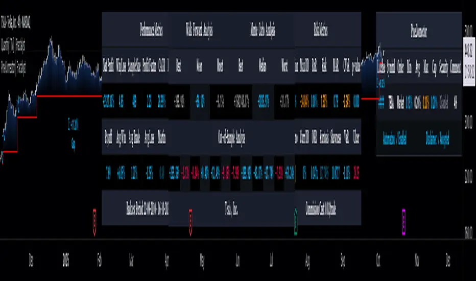
QuantFrame | FractalystWhat’s the purpose of this indicator?
The purpose of QuantFrame is to provide traders with a systematic approach to analyzing market structure, eliminating subjectivity, and enhancing decision-making. By clearly identifying and labeling structural breaks, QuantFrame helps traders:
1. Refine Market Analysis: Transition from discretionary market observation to a structured framework.
2. Identify Key Levels: Highlight important liquidity and invalidation zones for potential entries, exits, and risk management.
3. Streamline Multi-Timeframe Analysis: Track market trends and structural changes across different timeframes seamlessly.
4. Enhance Consistency: Reduce guesswork by following a rule-based methodology for identifying structural breaks.
How Does This Indicator Identify Market Structure?
1. Swing Detection
• The indicator identifies key swing points on the chart. These are local highs or lows where the price reverses direction, forming the foundation of market structure.
2. Structural Break Validation
• A structural break is flagged when a candle closes above a previous swing high (bullish) or below a previous swing low (bearish).
• Break Confirmation Process:
To confirm the break, the indicator applies the following rules:
• Valid Swing Preceding the Break: There must be at least one valid swing point before the break.
3. Numeric Labeling
• Each confirmed structural break is assigned a unique numeric ID starting from 1.
• This helps traders track breaks sequentially and analyze how the market structure evolves over time.
4. Liquidity and Invalidation Zones
• For every confirmed structural break, the indicator highlights two critical zones:
1. Liquidity Zone (LIQ): Represents the structural liquidity level.
2. Invalidation Zone (INV): Acts as Invalidation point if the structure fails to hold.
What do the extremities show us on the charts?
When using QuantFrame for market structure analysis, the extremities—Liquidity Level (LIQ) and Invalidation Level (INV)—serve as critical reference points for understanding price behavior and making informed trading decisions.
Here's a detailed explanation of what these extremities represent and how they function:
Liquidity Level (LIQ)
Definition: The Liquidity Level is a key price zone where the market is likely to retest, consolidate, or seek liquidity. It represents areas where orders are concentrated, making it a high-probability reaction zone.
Purpose: Traders use this level to anticipate potential pullbacks or continuation patterns. It helps in identifying areas where price may pause or reverse temporarily due to the presence of significant liquidity.
Key Insight: If a candle closes above or below the LIQ, it results in another break of structure (BOS) in the same direction. This indicates that price is continuing its trend and has successfully absorbed liquidity at that level.
Invalidation Level (INV)
Definition: The Invalidation Level marks the threshold that, if breached, signifies a structural shift in the market. It acts as a critical point where the current market bias becomes invalid.
Purpose: This level is often used as a stop-loss or re-evaluation point for trading strategies. It ensures that traders have a clear boundary for risk management.
Key Insight: If a candle closes above or below the INV, it signals a shift in market structure:
A closure above the INV in a bearish trend indicates a shift from bearish to bullish bias.
A closure below the INV in a bullish trend indicates a shift from bullish to bearish bias.
What does the top table display?
The top table in QuantFrame serves as a multi-timeframe trend overview. Here’s what it provides:
1. Numeric Break IDs Across Multiple Timeframes:
• Each numeric break corresponds to a confirmed structural break on a specific timeframe, helping traders track the most recent breaks systematically.
2. Trend Direction via Text Color:
• The color of the text reflects the current trend direction:
• Blue indicates a bullish structure.
• Red signifies a bearish structure.
3. Higher Timeframe Insights Without Manual Switching:
• The table eliminates the need to switch between timeframes by presenting a consolidated view of the market trend across multiple timeframes, saving time and improving decision-making.
What is the Multi-Timeframe Trend Score (MTTS)?
MTTS is a score that quantifies trend strength and direction across multiple timeframes.
How does MTTS work?
1. Break Detection:
• Analyzes bullish and bearish structural breaks on each timeframe.
2. Trend Scoring:
• Scores each timeframe based on the frequency and quality of bullish/bearish breaks.
3. MTTS Calculation:
• Averages the scores across all timeframes to produce a unified trend strength value.
How is MTTS interpreted?
• ⬆ (Above 50): Indicates an overall bullish trend.
• ⬇ (Below 50): Suggests an overall bearish trend.
• ⇅ (Exactly 50): Represents a neutral or balanced market structure.
How to Use QuantFrame?
1. Implement a Systematic Market Structure Framework:
• Use QuantFrame to analyze market structure objectively by identifying key structural breaks and marking liquidity (LIQ) and invalidation (INV) zones.
• This eliminates guesswork and provides a clear framework for understanding market movements.
2. Leverage MTTS for Directional Bias:
• Refer to the MTTS table to identify the multi-timeframe directional bias, giving you the broader market context.
• Align your trading decisions with the overall trend or structure to improve accuracy and consistency.
3. Apply Your Preferred Entry Model:
• Once the market context is clear, use your preferred entry model to capitalize on the identified structure and trend.
• Manage trades dynamically as price delivers, using the provided liquidity and invalidation zones for risk management.
What Makes QuantFrame Original?
1. Objective Market Structure Analysis:
• Unlike subjective methods, QuantFrame uses a rule-based approach to identify structural breaks, ensuring consistency and reducing emotional decision-making.
2. Multi-Timeframe Integration:
• The MTTS table consolidates trend data across multiple timeframes, offering a bird’s-eye view of market trends without the need to switch charts manually.
• This unique feature allows traders to align strategies with higher-timeframe trends for more informed decision-making.
3. Liquidity and Invalidation Zones:
• Automatically marks Liquidity (LIQ) and Invalidation (INV) zones for every structural break, providing actionable levels for entries, exits, and risk management.
• These zones help traders define their risk-reward setups with precision.
4. Dynamic Trend Scoring (MTTS):
• The Multi-Timeframe Trend Score (MTTS) quantifies trend strength and direction across selected timeframes, offering a single, consolidated metric for market sentiment.
• This score is visualized with intuitive symbols (⬆, ⬇, ⇅) for quick decision-making.
5. Numeric Labeling of Breaks:
• Each structural break is assigned a unique numeric ID, making it easy to track, analyze, and backtest specific market scenarios.
6. Systematic Yet Flexible:
• While it provides a structured framework for market analysis, QuantFrame seamlessly integrates with any trading style. Traders can use it alongside their preferred entry models, adapting it to their unique strategies.
7. Enhanced Market Context:
• By combining structural insights with directional bias (via MTTS), the indicator equips traders with a complete market context, enabling them to make better-informed decisions.
Terms and Conditions | Disclaimer
Our charting tools are provided for informational and educational purposes only and should not be construed as financial, investment, or trading advice. They are not intended to forecast market movements or offer specific recommendations. Users should understand that past performance does not guarantee future results and should not base financial decisions solely on historical data.
Built-in components, features, and functionalities of our charting tools are the intellectual property of @Fractalyst use, reproduction, or distribution of these proprietary elements is prohibited.
By continuing to use our charting tools, the user acknowledges and accepts the Terms and Conditions outlined in this legal disclaimer and agrees to respect our intellectual property rights and comply with all applicable laws and regulations.
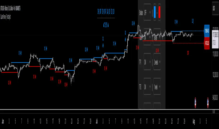
Quantify [Entry Model] | FractalystWhat’s the indicator’s purpose and functionality?
Quantify is a machine learning entry model designed to help traders identify high-probability setups to refine their strategies.
➙ Simply pick your bias, select your entry timeframes, and let Quantify handle the rest for you.
Can the indicator be applied to any market approach/trading strategy?
Absolutely, all trading strategies share one fundamental element: Directional Bias
Once you’ve determined the market bias using your own personal approach, whether it’s through technical analysis or fundamental analysis, select the trend direction in the Quantify user inputs.
The algorithm will then adjust its calculations to provide optimal entry levels aligned with your chosen bias. This involves analyzing historical patterns to identify setups with the highest potential expected values, ensuring your setups are aligned with the selected direction.
Can the indicator be used for different timeframes or trading styles?
Yes, regardless of the timeframe you’d like to take your entries, the indicator adapts to your trading style.
Whether you’re a swing trader, scalper, or even a position trader, the algorithm dynamically evaluates market conditions across your chosen timeframe.
How can this indicator help me to refine my trading strategy?
1. Focus on Positive Expected Value
• The indicator evaluates every setup to ensure it has a positive expected value, helping you focus only on trades that statistically favor long-term profitability.
2. Adapt to Market Conditions
• By analyzing real-time market behavior and historical patterns, the algorithm adjusts its calculations to match current conditions, keeping your strategy relevant and adaptable.
3. Eliminate Emotional Bias
• With clear probabilities, expected values, and data-driven insights, the indicator removes guesswork and helps you avoid emotional decisions that can damage your edge.
4. Optimize Entry Levels
• The indicator identifies optimal entry levels based on your selected bias and timeframes, improving robustness in your trades.
5. Enhance Risk Management
• Using tools like the Kelly Criterion, the indicator suggests optimal position sizes and risk levels, ensuring that your strategy maintains consistency and discipline.
6. Avoid Overtrading
• By highlighting only high-potential setups, the indicator keeps you focused on quality over quantity, helping you refine your strategy and avoid unnecessary losses.
How can I get started to use the indicator for my entries?
1. Set Your Market Bias
• Determine whether the market trend is Bullish or Bearish using your own approach.
• Select the corresponding bias in the indicator’s user inputs to align it with your analysis.
2. Choose Your Entry Timeframes
• Specify the timeframes you want to focus on for trade entries.
• The indicator will dynamically analyze these timeframes to provide optimal setups.
3. Let the Algorithm Analyze
• Quantify evaluates historical data and real-time price action to calculate probabilities and expected values.
• It highlights setups with the highest potential based on your selected bias and timeframes.
4. Refine Your Entries
• Use the insights provided—entry levels, probabilities, and risk calculations—to align your trades with a math-driven edge.
• Avoid overtrading by focusing only on setups with positive expected value.
5. Adapt to Market Conditions
• The indicator continuously adapts to real-time market behavior, ensuring its recommendations stay relevant and precise as conditions change.
How does the indicator calculate the current range?
The indicator calculates the current range by analyzing swing points from the very first bar on your charts to the latest available bar it identifies external liquidity levels, also known as BSLQ (buy-side liquidity levels) and SSLQ (sell-side liquidity levels).
What's the purpose of these levels? What are the underlying calculations?
1. Understanding Swing highs and Swing Lows
Swing High: A Swing High is formed when there is a high with 2 lower highs to the left and right.
Swing Low: A Swing Low is formed when there is a low with 2 higher lows to the left and right.
2. Understanding the purpose and the underlying calculations behind Buyside, Sellside and Pivot levels.
3. Identifying Discount and Premium Zones.
4. Importance of Risk-Reward in Premium and Discount Ranges
How does the script calculate probabilities?
The script calculates the probability of each liquidity level individually. Here's the breakdown:
1. Upon the formation of a new range, the script waits for the price to reach and tap into pivot level level. Status: "■" - Inactive
2. Once pivot level is tapped into, the pivot status becomes activated and it waits for either liquidity side to be hit. Status: "▶" - Active
3. If the buyside liquidity is hit, the script adds to the count of successful buyside liquidity occurrences. Similarly, if the sellside is tapped, it records successful sellside liquidity occurrences.
4. Finally, the number of successful occurrences for each side is divided by the overall count individually to calculate the range probabilities.
Note: The calculations are performed independently for each directional range. A range is considered bearish if the previous breakout was through a sellside liquidity. Conversely, a range is considered bullish if the most recent breakout was through a buyside liquidity.
What does the multi-timeframe functionality offer?
You can incorporate up to 4 higher timeframe probabilities directly into the table.
This feature allows you to analyze the probabilities of buyside and sellside liquidity across multiple timeframes, without the need to manually switch between them.
By viewing these higher timeframe probabilities in one place, traders can spot larger market trends and refine their entries and exits with a better understanding of the overall market context.
What are the multi-timeframe underlying calculations?
The script uses the same calculations (mentioned above) and uses security function to request the data such as price levels, bar time, probabilities and booleans from the user-input timeframe.
How does the Indicator Identifies Positive Expected Values?
Quantify instantly calculates whether a trade setup has the potential to generate positive expected value (EV).
To determine a positive EV setup, the indicator uses the formula:
EV = ( P(Win) × R(Win) ) − ( P(Loss) × R(Loss))
where:
- P(Win) is the probability of a winning trade.
- R(Win) is the reward or return for a winning trade, determined by the current risk-to-reward ratio (RR).
- P(Loss) is the probability of a losing trade.
- R(Loss) is the loss incurred per losing trade, typically assumed to be -1.
By calculating these values based on historical data and the current trading setup, the indicator helps you understand whether your trade has a positive expected value.
How can I know that the setup I'm going to trade with has a positive EV?
If the indicator detects that the adjusted pivot and buy/sell side probabilities have generated positive expected value (EV) in historical data, the risk-to-reward (RR) label within the range box will be colored blue and red .
If the setup does not produce positive EV, the RR label will appear gray.
This indicates that even the risk-to-reward ratio is greater than 1:1, the setup is not likely to yield a positive EV because, according to historical data, the number of losses outweighs the number of wins relative to the RR gain per winning trade.
What is the confidence level in the indicator, and how is it determined?
The confidence level in the indicator reflects the reliability of the probabilities calculated based on historical data. It is determined by the sample size of the probabilities used in the calculations. A larger sample size generally increases the confidence level, indicating that the probabilities are more reliable and consistent with past performance.
How does the confidence level affect the risk-to-reward (RR) label?
The confidence level (★) is visually represented alongside the probability label. A higher confidence level indicates that the probabilities used to determine the RR label are based on a larger and more reliable sample size.
How can traders use the confidence level to make better trading decisions?
Traders can use the confidence level to gauge the reliability of the probabilities and expected value (EV) calculations provided by the indicator. A confidence level above 95% is considered statistically significant and indicates that the historical data supporting the probabilities is robust. This high confidence level suggests that the probabilities are reliable and that the indicator’s recommendations are more likely to be accurate.
In data science and statistics, a confidence level above 95% generally means that there is less than a 5% chance that the observed results are due to random variation. This threshold is widely accepted in research and industry as a marker of statistical significance. Studies such as those published in the Journal of Statistical Software and the American Statistical Association support this threshold, emphasizing that a confidence level above 95% provides a strong assurance of data reliability and validity.
Conversely, a confidence level below 95% indicates that the sample size may be insufficient and that the data might be less reliable. In such cases, traders should approach the indicator’s recommendations with caution and consider additional factors or further analysis before making trading decisions.
How does the sample size affect the confidence level, and how does it relate to my TradingView plan?
The sample size for calculating the confidence level is directly influenced by the amount of historical data available on your charts. A larger sample size typically leads to more reliable probabilities and higher confidence levels.
Here’s how the TradingView plans affect your data access:
Essential Plan
The Essential Plan provides basic data access with a limited amount of historical data. This can lead to smaller sample sizes and lower confidence levels, which may weaken the robustness of your probability calculations. Suitable for casual traders who do not require extensive historical analysis.
Plus Plan
The Plus Plan offers more historical data than the Essential Plan, allowing for larger sample sizes and more accurate confidence levels. This enhancement improves the reliability of indicator calculations. This plan is ideal for more active traders looking to refine their strategies with better data.
Premium Plan
The Premium Plan grants access to extensive historical data, enabling the largest sample sizes and the highest confidence levels. This plan provides the most reliable data for accurate calculations, with up to 20,000 historical bars available for analysis. It is designed for serious traders who need comprehensive data for in-depth market analysis.
PRO+ Plans
The PRO+ Plans offer the most extensive historical data, allowing for the largest sample sizes and the highest confidence levels. These plans are tailored for professional traders who require advanced features and significant historical data to support their trading strategies effectively.
For many traders, the Premium Plan offers a good balance of affordability and sufficient sample size for accurate confidence levels.
What is the HTF probability table and how does it work?
The HTF (Higher Time Frame) probability table is a feature that allows you to view buy and sellside probabilities and their status from timeframes higher than your current chart timeframe.
Here’s how it works:
Data Request: The table requests and retrieves data from user-defined higher timeframes (HTFs) that you select.
Probability Display: It displays the buy and sellside probabilities for each of these HTFs, providing insights into the likelihood of price movements based on higher timeframe data.
Detailed Tooltips: The table includes detailed tooltips for each timeframe, offering additional context and explanations to help you understand the data better.
What do the different colors in the HTF probability table indicate?
The colors in the HTF probability table provide visual cues about the expected value (EV) of trading setups based on higher timeframe probabilities:
Blue: Suggests that entering a long position from the HTF user-defined pivot point, targeting buyside liquidity, is likely to result in a positive expected value (EV) based on historical data and sample size.
Red: Indicates that entering a short position from the HTF user-defined pivot point, targeting sellside liquidity, is likely to result in a positive expected value (EV) based on historical data and sample size.
Gray: Shows that neither long nor short trades from the HTF user-defined pivot point are expected to generate positive EV, suggesting that trading these setups may not be favorable.
What machine learning techniques are used in Quantify?
Quantify offers two main machine learning approaches:
1. Adaptive Learning (Fixed Sample Size): The algorithm learns from the entire dataset without resampling, maintaining a stable model that adapts to the latest market conditions.
2. Bootstrap Resampling: This method creates multiple subsets of the historical data, allowing the model to train on varying sample sizes. This technique enhances the robustness of predictions by ensuring that the model is not overfitting to a single dataset.
How does machine learning affect the expected value calculations in Quantify?
Machine learning plays a key role in improving the accuracy of expected value (EV) calculations. By analyzing historical price action, liquidity hits, and market bias patterns, the model continuously adjusts its understanding of risk and reward, allowing the expected value to reflect the most likely market movements. This results in more precise EV predictions, helping traders focus on setups that maximize profitability.
What is the Kelly Criterion, and how does it work in Quantify?
The Kelly Criterion is a mathematical formula used to determine the optimal position size for each trade, maximizing long-term growth while minimizing the risk of large drawdowns. It calculates the percentage of your portfolio to risk on a trade based on the probability of winning and the expected payoff.
Quantify integrates this with user-defined inputs to dynamically calculate the most effective position size in percentage, aligning with the trader’s risk tolerance and desired exposure.
How does Quantify use the Kelly Criterion in practice?
Quantify uses the Kelly Criterion to optimize position sizing based on the following factors:
1. Confidence Level: The model assesses the confidence level in the trade setup based on historical data and sample size. A higher confidence level increases the suggested position size because the trade has a higher probability of success.
2. Max Allowed Drawdown (User-Defined): Traders can set their preferred maximum allowed drawdown, which dictates how much loss is acceptable before reducing position size or stopping trading. Quantify uses this input to ensure that risk exposure aligns with the trader’s risk tolerance.
3. Probabilities: Quantify calculates the probabilities of success for each trade setup. The higher the probability of a successful trade (based on historical price action and liquidity levels), the larger the position size suggested by the Kelly Criterion.
What is a trailing stoploss, and how does it work in Quantify?
A trailing stoploss is a dynamic risk management tool that moves with the price as the market trend continues in the trader’s favor. Unlike a fixed take profit, which stays at a set level, the trailing stoploss automatically adjusts itself as the market moves, locking in profits as the price advances.
In Quantify, the trailing stoploss is enhanced by incorporating market structure liquidity levels (explain above). This ensures that the stoploss adjusts intelligently based on key price levels, allowing the trader to stay in the trade as long as the trend remains intact, while also protecting profits if the market reverses.
Why would a trader prefer a trailing stoploss based on liquidity levels instead of a fixed take-profit level?
Traders who use trailing stoplosses based on liquidity levels prefer this method because:
1. Market-Driven Flexibility: The stoploss follows the market structure rather than being static at a pre-defined level. This means the stoploss is less likely to be hit by small market fluctuations or false reversals. The stoploss remains adaptive, moving as the market moves.
2. Riding the Trend: Traders can capture more profit during a sustained trend because the trailing stop will adjust only when the trend starts to reverse significantly, based on key liquidity levels. This allows them to hold positions longer without prematurely locking in profits.
3. Avoiding Premature Exits: Fixed stoploss levels may exit a trade too early in volatile markets, while liquidity-based trailing stoploss levels respect the natural flow of price action, preventing the trader from exiting too soon during pullbacks or minor retracements.
🎲 Becoming the House: Gaining an Edge Over the Market
In American roulette, the casino has a 5.26% edge due to the presence of the 0 and 00 pockets. On even-money bets, players face a 47.37% chance of winning, while true 50/50 odds would require a 50% chance. This edge—the gap between the payout odds and the true probabilities—ensures that, statistically, the casino will always win over time, even if individual players win occasionally.
From a Trader’s Perspective
In trading, your edge comes from identifying and executing setups with a positive expected value (EV). For example:
• If you identify a setup with a 55.48% chance of winning and a 1:1 risk-to-reward (RR) ratio, your trade has a statistical advantage over a neutral (50/50) probability.
This edge works in your favor when applied consistently across a series of trades, just as the casino’s edge ensures profitability across thousands of spins.
🎰 Applying the Concept to Trading
Like casinos leverage their mathematical edge in games of chance, you can achieve long-term success in trading by focusing on setups with positive EV and managing your trades systematically. Here’s how:
1. Probability Advantage: Prioritize trades where the probability of success (win rate) exceeds the breakeven rate for your chosen risk-to-reward ratio.
• Example: With a 1:1 RR, you need a win rate above 50% to achieve positive EV.
2. Risk-to-Reward Ratio (RR): Even with a win rate below 50%, you can gain an edge by increasing your RR (e.g., a 40% win rate with a 2:1 RR still has positive EV).
3. Consistency and Discipline: Just as casinos profit by sticking to their mathematical advantage over thousands of spins, traders must rely on their edge across many trades, avoiding emotional decisions or overleveraging.
By targeting favorable probabilities and managing trades effectively, you “become the house” in your trading. This approach allows you to leverage statistical advantages to enhance your overall performance and achieve sustainable profitability.
What Makes the Quantify Indicator Original?
1. Data-Driven Edge
Unlike traditional indicators that rely on static formulas, Quantify leverages probability-based analysis and machine learning. It calculates expected value (EV) and confidence levels to help traders identify setups with a true statistical edge.
2. Integration of Market Structure
Quantify uses market structure liquidity levels to dynamically adapt. It identifies key zones like swing highs/lows and liquidity traps, enabling users to align entries and exits with where the market is most likely to react. This bridges the gap between price action analysis and quantitative trading.
3. Sophisticated Risk Management
The Kelly Criterion implementation is unique. Quantify allows traders to input their maximum allowed drawdown, dynamically adjusting risk exposure to maintain optimal position sizing. This ensures risk is scientifically controlled while maximizing potential growth.
4. Multi-Timeframe and Liquidity-Based Trailing Stops
The indicator doesn’t just suggest fixed profit-taking levels. It offers market structure-based trailing stop-loss functionality, letting traders ride trends as long as liquidity and probabilities favor the position, which is rare in most tools.
5. Customizable Bias and Adaptive Learning
• Directional Bias: Traders can set a bullish or bearish bias, and the indicator recalculates probabilities to align with the trader’s market outlook.
• Adaptive Learning: The machine learning model adapts to changes in data (via resampling or bootstrap methods), ensuring that predictions stay relevant in evolving markets.
6. Positive EV Focus
The focus on positive EV setups differentiates it from reactive indicators. It shifts trading from chasing signals to acting on setups that statistically favor profitability, akin to how professional quant funds operate.
7. User Empowerment
Through features like customizable timeframes, real-time probability updates, and visualization tools, Quantify empowers users to make data-informed decisions.
Terms and Conditions | Disclaimer
Our charting tools are provided for informational and educational purposes only and should not be construed as financial, investment, or trading advice. They are not intended to forecast market movements or offer specific recommendations. Users should understand that past performance does not guarantee future results and should not base financial decisions solely on historical data.
Built-in components, features, and functionalities of our charting tools are the intellectual property of @Fractalyst use, reproduction, or distribution of these proprietary elements is prohibited.
By continuing to use our charting tools, the user acknowledges and accepts the Terms and Conditions outlined in this legal disclaimer and agrees to respect our intellectual property rights and comply with all applicable laws and regulations.
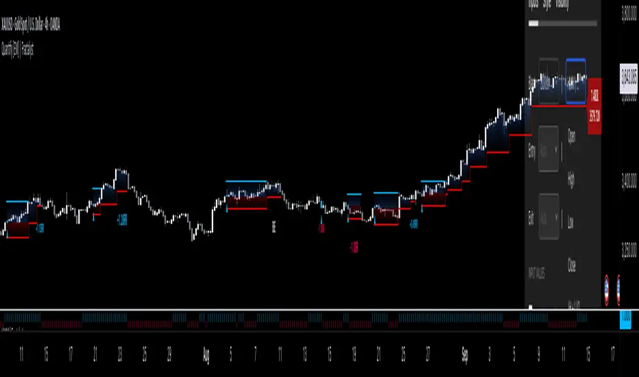
OrderFlow [Adjustable] | FractalystWhat's the indicator's purpose and functionality?
This indicator is designed to assist traders in identifying real-time probabilities of buyside and sellside liquidity .
It allows for an adjustable pivot level , enabling traders to customize the level they want to use for their entries.
By doing so, traders can evaluate whether their chosen entry point would yield a positive expected value over a large sample size, optimizing their strategy for long-term profitability.
For advanced traders looking to enhance their analysis, the indicator supports the incorporation of up to 7 higher timeframe biases .
Additionally, the higher timeframe pivot level can be adjusted according to the trader's preferences,
Offering maximum adaptability to different strategies and needs, further helping to maximize positive EV.
EV=(P(Win)×R(Win))−(P(Loss)×R(Loss))
-----
What's the purpose of these levels? What are the underlying calculations?
1. Understanding Swing highs and Swing Lows
Swing High: A Swing High is formed when there is a high with 2 lower highs to the left and right.
Swing Low: A Swing Low is formed when there is a low with 2 higher lows to the left and right.
2. Understanding the purpose and the underlying calculations behind Buyside, Sellside and Pivot levels.
3. Identifying Discount and Premium Zones.
4. Importance of Risk-Reward in Premium and Discount Ranges
----
How does the script calculate probabilities?
The script calculates the probability of each liquidity level individually. Here's the breakdown:
1. Upon the formation of a new range, the script waits for the price to reach and tap into pivot level level. Status: "⏸" - Inactive
2. Once pivot level is tapped into, the pivot status becomes activated and it waits for either liquidity side to be hit. Status: "▶" - Active
3. If the buyside liquidity is hit, the script adds to the count of successful buyside liquidity occurrences. Similarly, if the sellside is tapped, it records successful sellside liquidity occurrences.
4. Finally, the number of successful occurrences for each side is divided by the overall count individually to calculate the range probabilities.
Note: The calculations are performed independently for each directional range. A range is considered bearish if the previous breakout was through a sellside liquidity. Conversely, a range is considered bullish if the most recent breakout was through a buyside liquidity.
----
What does the multi-timeframe functionality offer?
In the adjustable version of the orderflow indicator, you can incorporate up to 7 higher timeframe probabilities directly into the table.
This feature allows you to analyze the probabilities of buyside and sellside liquidity across multiple timeframes, without the need to manually switch between them.
By viewing these higher timeframe probabilities in one place, traders can spot larger market trends and refine their entries and exits with a better understanding of the overall market context.
This multi-timeframe functionality helps traders:
1. Simplify decision-making by offering a comprehensive view of multiple timeframes at once.
2. Identify confluence between timeframes, enhancing the confidence in trade setups.
3. Adapt strategies more effectively, as the higher timeframe pivot levels can be customized to meet individual preferences and goals.
----
What are the multi-timeframe underlying calculations?
The script uses the same calculations (mentioned above) and uses security function to request the data such as price levels, bar time, probabilities and booleans from the user-input timeframe.
----
How does the Indicator Identifies Positive Expected Values?
OrderFlow indicator instantly calculates whether a trade setup has the potential for positive expected value (EV) in the long run.
To determine a positive EV setup, the indicator uses the formula:
EV=(P(Win)×R(Win))−(P(Loss)×R(Loss))
where:
P(Win) is the probability of a winning trade.
R(Win) is the reward or return for a winning trade, determined by the current risk-to-reward ratio (RR).
P(Loss) is the probability of a losing trade.
R(Loss) is the loss incurred per losing trade, typically assumed to be -1.
By calculating these values based on historical data and the current trading setup, the indicator helps you understand whether your trade has a positive expected value over a large sample size.
----
How can I know that the setup I'm going to trade with has a postive EV?
If the indicator detects that the adjusted pivot and buy/sell side probabilities have generated positive expected value (EV) in historical data, the risk-to-reward (RR) label within the range box will be colored blue and red .
If the setup does not produce positive EV, the RR label will appear gray.
This indicates that even the risk-to-reward ratio is greater than 1:1, the setup is not likely to yield a positive EV because, according to historical data, the number of losses outweighs the number of wins relative to the RR gain per winning trade.
----
What is the confidence level in the indicator, and how is it determined?
The confidence level in the indicator reflects the reliability of the probabilities calculated based on historical data. It is determined by the sample size of the probabilities used in the calculations. A larger sample size generally increases the confidence level, indicating that the probabilities are more reliable and consistent with past performance.
----
How does the confidence level affect the risk-to-reward (RR) label?
The confidence level (★) is visually represented alongside the probability label. A higher confidence level indicates that the probabilities used to determine the RR label are based on a larger and more reliable sample size.
----
How can traders use the confidence level to make better trading decisions?
Traders can use the confidence level to gauge the reliability of the probabilities and expected value (EV) calculations provided by the indicator. A confidence level above 95% is considered statistically significant and indicates that the historical data supporting the probabilities is robust. This high confidence level suggests that the probabilities are reliable and that the indicator’s recommendations are more likely to be accurate.
In data science and statistics, a confidence level above 95% generally means that there is less than a 5% chance that the observed results are due to random variation. This threshold is widely accepted in research and industry as a marker of statistical significance. Studies such as those published in the Journal of Statistical Software and the American Statistical Association support this threshold, emphasizing that a confidence level above 95% provides a strong assurance of data reliability and validity.
Conversely, a confidence level below 95% indicates that the sample size may be insufficient and that the data might be less reliable . In such cases, traders should approach the indicator’s recommendations with caution and consider additional factors or further analysis before making trading decisions.
----
How does the sample size affect the confidence level, and how does it relate to my TradingView plan?
The sample size for calculating the confidence level is directly influenced by the amount of historical data available on your charts. A larger sample size typically leads to more reliable probabilities and higher confidence levels.
Here’s how the TradingView plans affect your data access:
Essential Plan
The Essential Plan provides basic data access with a limited amount of historical data. This can lead to smaller sample sizes and lower confidence levels, which may weaken the robustness of your probability calculations. Suitable for casual traders who do not require extensive historical analysis.
Plus Plan
The Plus Plan offers more historical data than the Essential Plan, allowing for larger sample sizes and more accurate confidence levels. This enhancement improves the reliability of indicator calculations. This plan is ideal for more active traders looking to refine their strategies with better data.
Premium Plan
The Premium Plan grants access to extensive historical data, enabling the largest sample sizes and the highest confidence levels. This plan provides the most reliable data for accurate calculations, with up to 20,000 historical bars available for analysis. It is designed for serious traders who need comprehensive data for in-depth market analysis.
PRO+ Plans
The PRO+ Plans offer the most extensive historical data, allowing for the largest sample sizes and the highest confidence levels. These plans are tailored for professional traders who require advanced features and significant historical data to support their trading strategies effectively.
For many traders, the Premium Plan offers a good balance of affordability and sufficient sample size for accurate confidence levels.
----
What is the HTF probability table and how does it work?
The HTF (Higher Time Frame) probability table is a feature that allows you to view buy and sellside probabilities and their status from timeframes higher than your current chart timeframe.
Here’s how it works:
Data Request : The table requests and retrieves data from user-defined higher timeframes (HTFs) that you select.
Probability Display: It displays the buy and sellside probabilities for each of these HTFs, providing insights into the likelihood of price movements based on higher timeframe data.
Detailed Tooltips: The table includes detailed tooltips for each timeframe, offering additional context and explanations to help you understand the data better.
----
What do the different colors in the HTF probability table indicate?
The colors in the HTF probability table provide visual cues about the expected value (EV) of trading setups based on higher timeframe probabilities:
Blue: Suggests that entering a long position from the HTF user-defined pivot point, targeting buyside liquidity, is likely to result in a positive expected value (EV) based on historical data and sample size.
Red: Indicates that entering a short position from the HTF user-defined pivot point, targeting sellside liquidity, is likely to result in a positive expected value (EV) based on historical data and sample size.
Gray: Shows that neither long nor short trades from the HTF user-defined pivot point are expected to generate positive EV, suggesting that trading these setups may not be favorable.
----
How to use the indicator effectively?
For Amateur Traders:
Start Simple: Begin by focusing on one timeframe at a time with the pivot level set to the default (50%). This helps you understand the basic functionality of the indicator.
Entry and Exit Strategy: Focus on entering trades at the pivot level while targeting the higher probability side for take profit and the lower probability side for stop loss.
Use simulation or paper trading to practice this strategy.
Adjustments: Once you have a solid understanding of how the indicator works, you can start adjusting the pivot level to other values that suit your strategy.
Ensure that the RR labels are colored (blue or red) to indicate positive EV setups before executing trades.
For Advanced Traders:
1. Select Higher Timeframe Bias: Choose a higher timeframe (HTF) as your main bias. Start with the default pivot level and ensure the confidence level is above 95% to validate the probabilities.
2. Align Lower Timeframes: Switch between lower timeframes to identify which ones align with your predefined HTF bias. This helps in synchronizing your trading decisions across different timeframes.
3. Set Entries with Current Pivot Level: Use the current pivot level for trade entries. Ensure the HTF status label is active, indicating that the probabilities are valid and in play.
4. Target HTF Liquidity Level: Aim for liquidity levels that correspond to the higher timeframe, as these levels are likely to offer better trading opportunities.
5. Adjust Pivot Levels: As you gain experience, adjust the pivot levels to further optimize your strategy for high EV. Fine-tune these levels based on the aggregated data from multiple timeframes.
6. Practice on Paper Trading: Test your strategies through paper trading to eliminate discretion and refine your approach without financial risk.
7. Focus on Trade Management: Ultimately, effective trade management is crucial. Concentrate on managing your trades well to ensure long-term success. By aiming for setups that produce positive EV, you can position yourself similarly to how a casino operates.
----
🎲 Becoming the House (Gaining Edge Over the Market):
In American roulette, the house has a 5.26% edge due to the 0 and 00. This means that while players have a 47.37% chance of winning on even-money bets, the true odds are 50%. The discrepancy between the true odds and the payout ensures that, statistically, the casino will win over time.
From the Trader's Perspective: In trading, you gain an edge by focusing on setups with positive expected value (EV). If you have a 55.48% chance of winning with a 1:1 risk-to-reward ratio, your setup has a higher probability of profitability than the losing side. By consistently targeting such setups and managing your trades effectively, you create a statistical advantage, similar to the casino’s edge.
----
🎰 Applying the Concept to Trading:
Just as casinos rely on their mathematical edge, you can achieve long-term success in trading by focusing on setups with positive EV. By ensuring that your probabilities and risk-to-reward (RR) ratios are in your favor, you create an edge similar to that of the house.
And by systematically targeting trades with favorable probabilities and managing your trades effectively, you improve your chances of profitability over the long run. Which is going to help you “become the house” in your trading, leveraging statistical advantages to enhance your overall performance.
----
What makes this indicator original?
Real-Time Probability Calculations: The indicator provides real-time calculations of buy and sell probabilities based on historical data, allowing traders to assess the likelihood of positive expected value (EV) setups instantly.
Adjustable Pivot Levels: It features an adjustable pivot level that traders can modify according to their preferences, enhancing the flexibility to align with different trading strategies.
Multi-Timeframe Integration: The indicator supports up to 7 higher timeframes, displaying their probabilities and biases in a single view, which helps traders make informed decisions without switching timeframes.
Confidence Levels: It includes confidence levels based on sample sizes, offering insights into the reliability of the probabilities. Traders can gauge the strength of the data before making trades.
Dynamic EV Labels: The indicator provides color-coded EV labels that change based on the validity of the setup. Blue indicates positive EV in a long bias, red indicates positive EV in a short bias and gray signals caution, making it easier for traders to identify high-quality setups.
HTF Probability Table: The HTF probability table displays buy and sell probabilities from user-defined higher timeframes, helping traders integrate broader market context into their decision-making process.
----
Terms and Conditions | Disclaimer
Our charting tools are provided for informational and educational purposes only and should not be construed as financial, investment, or trading advice. They are not intended to forecast market movements or offer specific recommendations. Users should understand that past performance does not guarantee future results and should not base financial decisions solely on historical data.
Built-in components, features, and functionalities of our charting tools are the intellectual property of @Fractalyst use, reproduction, or distribution of these proprietary elements is prohibited.
By continuing to use our charting tools, the user acknowledges and accepts the Terms and Conditions outlined in this legal disclaimer and agrees to respect our intellectual property rights and comply with all applicable laws and regulations.

Matrix Glitch | FractalystThe Matrix Glitch indicator is a visually engaging tool for traders, inspired by the iconic Matrix movie effects. It overlays price charts with dynamic, multi-colored glitches that sync with market data, creating a striking, almost surreal visual experience.
The indicator uses characters from various languages (e.g., Japanese, Chinese, Russian, English) to mimic the digital rain effect from the movies. Users can select a language, which activates a corresponding array of characters. These characters are randomly picked from the chosen array and displayed on the chart.
Underlying Calculations and Logic
Arrays in the Indicator
1- Character Management:
The script uses arrays to store sets of characters representing different symbols or alphabets. These arrays allow the indicator to dynamically select and update characters for display. Each element in these arrays corresponds to a specific character that will be used to populate the grid.
2- Current and Previous States:
Arrays are employed to keep track of the current state of characters that are displayed on the grid. Simultaneously, another set of arrays records the previous state of these characters. This dual-state management allows the script to smoothly transition between updates, handling changes in characters and visual effects like fading.
3- Transparency Control:
Transparency levels for each character in the grid are managed through arrays. These arrays store the opacity values, ensuring that each character has the appropriate level of transparency. By comparing the current and previous transparency states, the script can create effects like gradual fading or intensifying visibility.
4- Rain Effect Simulation:
To create the "rain" effect, the script maintains arrays that simulate the falling text by continuously updating the position and visibility of characters. As new characters enter the top of the grid, older ones are removed from the bottom, with their transparency levels adjusted to simulate movement.
5- Operational Flow:
Initialization : Arrays are initialized to manage both the characters and their transparency. This setup allows the script to handle the dynamic display efficiently.
Updates : During each cycle, new characters are selected and old characters are shifted accordingly. The arrays ensure that both the content and appearance of the grid are updated seamlessly.
Rendering : The arrays dictate how characters and their transparency are rendered on the grid, ensuring a cohesive and visually appealing effect.
Here's how to use the indicator step-by-step:
1- Apply the Indicator to Your Charts:
Begin by adding the indicator to your chart. This will activate the visual effect on your selected trading instrument or time frame.
Select Your Preferred Language of the Matrix Characters:
In the settings, choose the language or symbol set you want the matrix characters to display. This could be anything from traditional matrix-style characters to different alphabets or custom symbols.
2- Choose the Matrix Effect (Rain, Burst):
Decide on the type of visual effect you prefer. You can select from options like the classic "rain" effect, where characters fall from the top of the screen, or a "burst" effect, where characters explode outward or appear in a different dynamic pattern.
3- Adjust the Color According to Your Preference:
Customize the color of the matrix characters to suit your aesthetic or chart theme. You can select from a range of colors or even set up a gradient for more complex visual effects.
4- Adjust the Width and Height of the Matrix According to Your Screen:
Fine-tune the dimensions of the matrix display. Set the width and height so that the matrix fits perfectly on your screen, ensuring that it aligns well with other chart elements and doesn't obstruct your view.
------
What Makes the Matrix Glitch Indicator Unique?
Language Selection:
Customizable Language: Unlike many indicators that might offer static or limited visual elements, the Matrix Glitch Indicator allows users to choose from a variety of languages for the characters displayed. This feature not only personalizes the user experience but also adds a cultural or linguistic element to trading charts. Users can select languages like Japanese, Chinese, Russian, or English, and many more.
This flexibility ensures that traders from different backgrounds can feel a connection with their charts through familiar or exotic scripts.
Dynamic Effects:
Effect Modes: The indicator offers two distinct modes - Rain Mode and Burst Mode. In Rain Mode, characters fall from the top of the chart, mimicking the iconic digital rain from the Matrix films.
In Burst Mode, characters radiate outward from a central point, creating a unique visual effect that can be synchronized with market volatility.
This dual-mode functionality allows traders to choose how they want their data to be visually represented, providing both aesthetic variety and potentially different insights into market behavior.
Color Customization:
Full Color Control: The ability to fully customize the color of the characters is a standout feature. Traders can match the indicator's colors to their trading platform's theme, their mood, or even specific market conditions (e.g., red for downturns, green for upturns). This level of customization not only aids in creating a personalized trading environment but can also serve as a visual cue for different market states.
Universal Display Compatibility:
Adjustability for All Displays: The indicator is designed to be fully adjustable for various screen resolutions and sizes. This ensures that whether you're trading on a high-resolution monitor, a laptop, or even a mobile device, the Matrix Glitch effect remains clear and impactful without compromising on the functionality of the trading chart. This adaptability is crucial in an era where trading can happen anywhere, making the indicator a versatile tool for traders on the go or in a static setup.
------
Terms and Conditions | Disclaimer
Our charting tools are provided for informational and educational purposes only and should not be construed as financial, investment, or trading advice. They are not intended to forecast market movements or offer specific recommendations. Users should understand that past performance does not guarantee future results and should not base financial decisions solely on historical data.
Built-in components, features, and functionalities of our charting tools are the intellectual property of @Fractalyst use, reproduction, or distribution of these proprietary elements is prohibited.
By continuing to use our charting tools, the user acknowledges and accepts the Terms and Conditions outlined in this legal disclaimer and agrees to respect our intellectual property rights and comply with all applicable laws and regulations.

Range Sentiment | FractalystWhat’s the purpose of this indicator?
This indicator aims to calculate the percentage level of bullish or bearish fluctuations within equally divided price sections, in the latest price range.
----
How does this indicator calculate the current sentiment?
This indicator calculates the current sentiment by identifying the highest swing high and the lowest swing low, then evenly dividing the distance between them into percentage amounts. If the price is above the 50% mark, it indicates bullishness, whereas if it's below 50%, it suggests bearishness.
----
Is this sentiment the same as the ones on online websites?
No, the sentiment as discussed earlier, is based on analyzing price action on charts and calculating the current range in percentage.
----
What methods do other websites typically use to determine market sentiment?
1. Broker Data Aggregation: Compiling data from various forex brokers to assess the percentage of long and short positions taken by traders.
2. Lot Size Analysis: Considering the size of positions taken by traders, where a significant number of large positions in one direction may indicate strong bullish or bearish sentiment.
3. Order Flow Analysis: Tracking the flow of orders in the forex market, with an increase in buy orders suggesting bullish sentiment and a surge in sell orders indicating bearish sentiment.
4. Sentiment Surveys: Conducting surveys among forex traders to gather opinions about future price movements and gauge sentiment.
----
What are the options to display the current market sentiment?
1. Table - located at top centre of your charts
2. Label - indicating the 50% level of the current range mentioned above
----
How can I analyze how the sentiment worked on historical data?
There are 3 available options:
1. Shapes
2. Candles
3. Background
- White colour/transparent background denote a weak or uncertain trend, where the bullish or bearish degree is less than 60%.
- Blue colour indicates that the price is trading bullish.
- Red colour indicates that the price is trading bearish.
----
On what market and timeframe this indicator operates on?
The Range Sentiment indicator is applicable to all markets and timeframes.
When switching between timeframes, the values remain consistent because it utilizes the daily bias to determine the sentiment for the current day.
----
How can I use this indicator?
1. Add "Range Sentiment | Fractalyst" to your TradingView chart.
2. Choose the pair you want to analyze or trade intraday/during session.
3. Make sure the sentiment is showing you a bullish or a bearish degree of higher than 60%.
(To avoid potentially choppy price action)
4. Use your favourite entry model to trade in the same direction that the sentiment is showing you.
5. Determine your take profit based on the daily swing level OR previous daily high if the bullish degree is above +60% and previous daily low if the bearish degree is +60%.
6. Risk adjustment and Trade management based on your personal preferences.
Example:
----
User-input settings and customizations
----
What makes this indicator original?
1. It utilizes the daily timeframe's current range to determine the day's bias degree in percentage.
2. Apart from presenting the current sentiment in a sentimental table, it also visualizes the 50% threshold as a label, indicating where price may shift direction from a sentiment perspective.
3. It offers the feature to analyze historical data, allowing users to observe indicator performance through shapes, candles, and background colors.
4. By integrating market sentiment directly into the charts, it simplifies the trading process, removing the reliance on online websites and services for sentiment analysis, which often rely on limited brokerage data and resources.
5. Unlike most sentiment websites that primarily focus on forex pairs sentiment data, this indicator stands out by its capability to analyze sentiment across all markets. Moreover, it provides real-time updates, ensuring traders have access to the latest sentiment information regardless of the market they are trading in.
----
Terms and Conditions | Disclaimer
Our charting tools are provided for informational and educational purposes only and should not be construed as financial, investment, or trading advice. They are not intended to forecast market movements or offer specific recommendations. Users should understand that past performance does not guarantee future results and should not base financial decisions solely on historical data.
By continuing to use our charting tools, the user acknowledges and accepts the Terms and Conditions outlined in this legal disclaimer.