Adaptive Look-back/Volatility Phase Change Index on Jurik [Loxx]Adaptive Look-back, Adaptive Volatility Phase Change Index on Jurik is a Phase Change Index but with adaptive length and volatility inputs to reduce phase change noise and better identify trends. This is an invese indicator which means that small values on the oscillator indicate bullish sentiment and higher values on the oscillator indicate bearish sentiment
What is the Phase Change Index?
Based on the M.H. Pee's TASC article "Phase Change Index".
Prices at any time can be up, down, or unchanged. A period where market prices remain relatively unchanged is referred to as a consolidation. A period that witnesses relatively higher prices is referred to as an uptrend, while a period of relatively lower prices is called a downtrend.
The Phase Change Index (PCI) is an indicator designed specifically to detect changes in market phases.
This indicator is made as he describes it with one deviation: if we follow his formula to the letter then the "trend" is inverted to the actual market trend. Because of that an option to display inverted (and more logical) values is added.
What is the Jurik Moving Average?
Have you noticed how moving averages add some lag (delay) to your signals? ... especially when price gaps up or down in a big move, and you are waiting for your moving average to catch up? Wait no more! JMA eliminates this problem forever and gives you the best of both worlds: low lag and smooth lines.
Ideally, you would like a filtered signal to be both smooth and lag-free. Lag causes delays in your trades, and increasing lag in your indicators typically result in lower profits. In other words, late comers get what's left on the table after the feast has already begun.
That's why investors, banks and institutions worldwide ask for the Jurik Research Moving Average ( JMA ). You may apply it just as you would any other popular moving average. However, JMA's improved timing and smoothness will astound you.
What is adaptive Jurik volatility
One of the lesser known qualities of Juirk smoothing is that the Jurik smoothing process is adaptive. "Jurik Volty" (a sort of market volatility ) is what makes Jurik smoothing adaptive. The Jurik Volty calculation can be used as both a standalone indicator and to smooth other indicators that you wish to make adaptive.
What is an adaptive cycle, and what is Ehlers Autocorrelation Periodogram Algorithm?
From his Ehlers' book Cycle Analytics for Traders Advanced Technical Trading Concepts by John F. Ehlers, 2013, page 135:
"Adaptive filters can have several different meanings. For example, Perry Kaufman’s adaptive moving average (KAMA) and Tushar Chande’s variable index dynamic average (VIDYA) adapt to changes in volatility. By definition, these filters are reactive to price changes, and therefore they close the barn door after the horse is gone.The adaptive filters discussed in this chapter are the familiar Stochastic, relative strength index (RSI), commodity channel index (CCI), and band-pass filter.The key parameter in each case is the look-back period used to calculate the indicator. This look-back period is commonly a fixed value. However, since the measured cycle period is changing, it makes sense to adapt these indicators to the measured cycle period. When tradable market cycles are observed, they tend to persist for a short while.Therefore, by tuning the indicators to the measure cycle period they are optimized for current conditions and can even have predictive characteristics.
The dominant cycle period is measured using the Autocorrelation Periodogram Algorithm. That dominant cycle dynamically sets the look-back period for the indicators. I employ my own streamlined computation for the indicators that provide smoother and easier to interpret outputs than traditional methods. Further, the indicator codes have been modified to remove the effects of spectral dilation.This basically creates a whole new set of indicators for your trading arsenal."
Included
-Your choice of length input calculation, either fixed or adaptive cycle
-Invert the signal to match the trend
-Bar coloring to paint the trend
Happy trading!
Recherche dans les scripts pour "algo"
Adaptive MA Difference constructor [lastguru]A complimentary indicator to my Adaptive MA constructor. It calculates the difference between the two MA lines (inspired by the Moving Average Difference (MAD) indicator by John F. Ehlers). You can then further smooth the resulting curve. The parameters and options are explained here:
The difference is normalized by dividing the difference by twice its Root mean square (RMS) over Slow MA length. Inverse Fisher Transform is then used to force the -1..1 range.
Same Postfilter options are provided as in my Adaptive Oscillator constructor:
Stochastic - Stochastic
Super Smooth Stochastic - Super Smooth Stochastic (part of MESA Stochastic ) by John F. Ehlers
Inverse Fisher Transform - Inverse Fisher Transform
Noise Elimination Technology - a simplified Kendall correlation algorithm "Noise Elimination Technology" by John F. Ehlers
Momentum - momentum (derivative)
Except for Inverse Fisher Transform, all Postfilter algorithms can have Length parameter. If it is not specified (set to 0), then the calculated Slow MA Length is used.
Mean Shift Pivot ClusteringCore Concepts
According to Jeff Greenblatt in his book "Breakthrough Strategies for Predicting Any Market", Fibonacci and Lucas sequences are observed repeated in the bar counts from local pivot highs/lows. They occur from high to high, low to high, high to low, or low to high. Essentially, this phenomenon is observed repeatedly from any pivot points on any time frame. Greenblatt combines this observation with Elliott Waves to predict the price and time reversals. However, I am no Elliottician so it was not easy for me to use this in a practical manner. I decided to only use the bar count projections and ignore the price. I projected a subset of Fibonacci and Lucas sequences along with the Fibonacci ratios from each pivot point. As expected, a projection from each pivot point resulted in a large set of plotted data and looks like a huge gong show of lines. Surprisingly, I did notice clusters and have observed those clusters to be fairly accurate.
Fibonacci Sequence: 1, 2, 3, 5, 8, 13, 21, 34...
Lucas Sequence: 2, 1, 3, 4, 7, 11, 18, 29, 47...
Fibonacci Ratios (converted to whole numbers): 23, 38, 50, 61, 78, 127, 161...
Light Bulb Moment
My eyes may suck at grouping the lines together but what about clustering algorithms? I chose to use a gimped version of Mean Shift because it doesn't require me to know in advance how many lines to expect like K-Means. Mean shift is computationally expensive and with Pinescript's 500ms timeout, I had to make due without the KDE. In other words, I skipped the weighting part but I may try to incorporate it in the future. The code is from Harrison Kinsley . He's a fantastic teacher!
Usage
Search Radius: how far apart should the bars be before they are excluded from the cluster? Try to stick with a figure between 1-5. Too large a figure will give meaningless results.
Pivot Offset: looks left and right X number of bars for a pivot. Same setting as the default TradingView pivot high/low script.
Show Lines Back: show historical predicted lines. (These can change)
Use this script in conjunction with Fibonacci price retracement/extension levels and/or other support/resistance levels. If it's no where near a support/resistance and there's a projected time pivot coming up, it's probably a fake out.
Notes
Re-painting is intended. When a new pivot is found, it will project out the Fib/Lucas sequences so the algorithm will run again with additional information.
The script is for informational and educational purposes only.
Do not use this indicator by itself to trade!
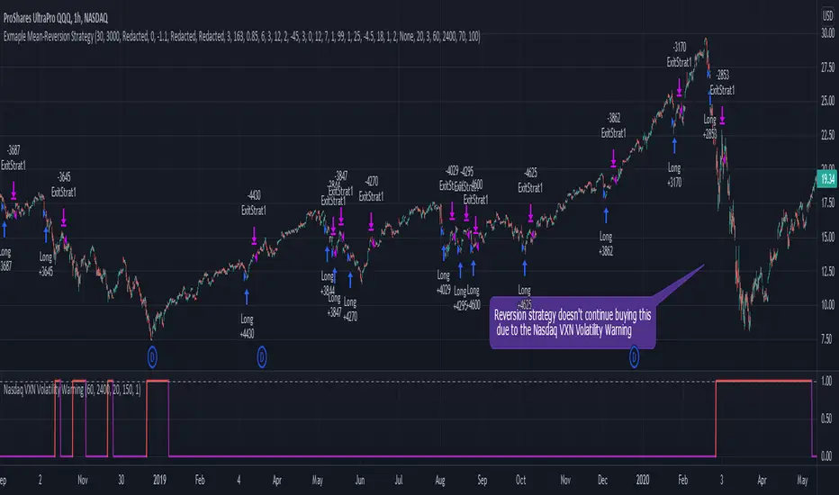
Nasdaq VXN Volatility Warning IndicatorToday I am sharing with the community a volatility indicator that uses the Nasdaq VXN Volatility Index to help you or your algorithms avoid black swan events. This is a similar the indicator I published last week that uses the SP500 VIX, but this indicator uses the Nasdaq VXN and can help inform strategies on the Nasdaq index or Nasdaq derivative instruments.
Variance is most commonly used in statistics to derive standard deviation (with its square root). It does have another practical application, and that is to identify outliers in a sample of data. Variance is defined as the squared difference between a value and its mean. Calculating that squared difference means that the farther away the value is from the mean, the more the variance will grow (exponentially). This exponential difference makes outliers in the variance data more apparent.
Why does this matter?
There are assets or indices that exist in the stock market that might make us adjust our trading strategy if they are behaving in an unusual way. In some instances, we can use variance to identify that behavior and inform our strategy.
Is that really possible?
Let’s look at the relationship between VXN and the Nasdaq100 as an example. If you trade a Nasdaq index with a mean reversion strategy or algorithm, you know that they typically do best in times of volatility . These strategies essentially attempt to “call bottom” on a pullback. Their downside is that sometimes a pullback turns into a regime change, or a black swan event. The other downside is that there is no logical tight stop that actually increases their performance, so when they lose they tend to lose big.
So that begs the question, how might one quantitatively identify if this dip could turn into a regime change or black swan event?
The Nasdaq Volatility Index ( VXN ) uses options data to identify, on a large scale, what investors overall expect the market to do in the near future. The Volatility Index spikes in times of uncertainty and when investors expect the market to go down. However, during a black swan event, historically the VXN has spiked a lot harder. We can use variance here to identify if a spike in the VXN exceeds our threshold for a normal market pullback, and potentially avoid entering trades for a period of time (I.e. maybe we don’t buy that dip).
Does this actually work?
In backtesting, this cut the drawdown of my index reversion strategies in half. It also cuts out some good trades (because high investor fear isn’t always indicative of a regime change or black swan event). But, I’ll happily lose out on some good trades in exchange for half the drawdown. Lets look at some examples of periods of time that trades could have been avoided using this strategy/indicator:
Example 1 – With the Volatility Warning Indicator, the mean reversion strategy could have avoided repeatedly buying this pullback that led to this asset losing over 75% of its value:
Example 2 - June 2018 to June 2019 - With the Volatility Warning Indicator, the drawdown during this period reduces from 22% to 11%, and the overall returns increase from -8% to +3%
How do you use this indicator?
This indicator determines the variance of VXN against a long term mean. If the variance of the VXN spikes over an input threshold, the indicator goes up. The indicator will remain up for a defined period of bars/time after the variance returns below the threshold. I have included default values I’ve found to be significant for a short-term mean-reversion strategy, but your inputs might depend on your risk tolerance and strategy time-horizon. The default values are for 1hr VXN data/charts. It will pull in variance data for the VXN regardless of which chart the indicator is applied to.
Disclaimer: Open-source scripts I publish in the community are largely meant to spark ideas or be used as building blocks for part of a more robust trade management strategy. If you would like to implement a version of any script, I would recommend making significant additions/modifications to the strategy & risk management functions. If you don’t know how to program in Pine, then hire a Pine-coder. We can help!
S&P500 VIX Volatility Warning IndicatorToday I am sharing with the community a volatility indicator that can help you or your algorithms avoid black swan events. Variance is most commonly used in statistics to derive standard deviation (with its square root). It does have another practical application, and that is to identify outliers in a sample of data. Variance in statistics is defined as the squared difference between a value and its mean. Calculating that squared difference means that the farther away the value is from the mean, the more the variance will grow (exponentially). This exponential difference makes outliers in the variance data more apparent.
Why does this matter?
There are assets or indices that exist in the stock market that might make us adjust our trading strategy if they are behaving in an unusual way. In some instances, we can use variance to identify that behavior and inform our strategy.
Is that really possible?
Let’s look at the relationship between VIX and the S&P500 as an example. If you trade an S&P500 index with a mean reversion strategy or algorithm, you know that they typically do best in times of volatility. These strategies essentially attempt to “call bottom” on a pullback. Their downside is that sometimes a pullback turns into a regime change, or a black swan event. The other downside is that there is no logical tight stop that actually increases their performance, so when they lose they tend to lose big.
So that begs the question, how might one quantitatively identify if this dip could turn into a regime change or black swan event?
The CBOE Volatility Index (VIX) uses options data to identify, on a large scale, what investors overall expect the market to do in the near future. The Volatility Index spikes in times of uncertainty and when investors expect the market to go down. However, during a black swan event, the VIX spikes a lot harder. We can use variance here to identify if a spike in the VIX exceeds our threshold for a normal market pullback, and potentially avoid entering trades for a period of time (I.e. maybe we don’t buy that dip).
Does this actually work?
In backtesting, this cut the drawdown of my index reversion strategies in half. It also cuts out some good trades (because high investor fear isn’t always indicative of a regime change or black swan event). But, I’ll happily lose out on some good trades in exchange for half the drawdown. Lets look at some examples of periods of time that trades could have been avoided using this strategy/indicator:
Example 1 – With the Volatility Warning Indicator, the mean reversion strategy could have avoided repeatedly buying this pullback that led to SPXL losing over 75% of its value:
Example 2 - June 2018 to June 2019 - With the Volatility Warning Indicator, the drawdown during this period reduces from 22% to 11%, and the overall returns increase from -8% to +3%
How do you use this indicator?
This indicator determines the variance of the VIX against a long term mean. If the variance of the VIX spikes over an input threshold, the indicator goes up. The indicator will remain up for a defined period of bars/time after the variance returns below the threshold. I have included default values I’ve found to be significant for a short-term mean-reversion strategy, but your inputs might depend on your risk tolerance and strategy time-horizon. The default values are for 1hr VIX data. It will pull in variance data for the VIX regardless of which chart the indicator is applied to.
Disclaimer : Open-source scripts I publish in the community are largely meant to spark ideas or be used as building blocks for part of a more robust trade management strategy. If you would like to implement a version of any script, I would recommend making significant additions/modifications to the strategy & risk management functions. If you don’t know how to program in Pine, then hire a Pine-coder. We can help!

Total VolumeThis simple indicator unifies the volumes of multiple exchanges/brokers. The idea of this indicator stems from the need to monitor the movements made by whales on other markets that can actually influence the price (manipulations, arbitrage, etc.).
Basically, we can:
* choose the number and symbols
* choose with which algorithm to merge the volumes (sum, average, weighted average, maximum)
* color the histogram (based on the dominant exchange, classic green/red color, no color)
Furthermore, there is a summary table which, in addition to indicating the volume for each exchange, also indicates the color attributed.
you can see the volume of the current exchange behind the volume obtained by the algorithm.
If you have any questions, doubts or suggestions please write to me.

Pulu's Moving AveragesPulu's Moving Averages
This script allows you to customize sets of moving averages. It is configured default as 3 Vegas tunnels + an MA12. You can re-configure it for any of your moving average studies. At the first release, it supports up to 7 moving averages, many parameters, and eight types of algorithms:
ALMA, Arnaud Legoux Moving Average
EMA, Exponential Moving Average
RMA, Adjusted exponential moving average (aka Wilder’s EMA)
SMA, Simple Moving Average
SWMA, Symmetrically-Weighted Moving Average
VWAP, Volume-Weighted Average Price
VWMA, Volume-Weighted Moving Average
WMA, Weighted Moving Average
If you are looking for only 3 moving averages, there is another script "Pulu's 3 Moving Averages".
Vigia blai5VIGÍA is the latest and current version of this weighted indicator that collects, combines and harmonizes the values of four other classic indicators: RSI, MFI, Bollinger Bands and Stochastic.
It is a 2nd Generation indicator, as it does not base its algorithm on pure price data, but on its evolution (volatility, volume differences, power variations, cycle phase ...) working from first generation indicators included and mixed in the algorithm.
With the RSI we detect current power or depletion; the MFI adds the harmonization between price and volume; Bollinger Bands warn us of positions in areas close to support and resistance, and Stochastic informs us of the favorable and unfavorable phases of its cycle. VIGÍA tries to gather all this information in a single value and signal. This is how the curve of this indicator emerges.
The layout of this curve is its own and different from that of the other four separately. But the key idea of this complex indicator is to harmonize the signals.
By "harmonizing" we mean that an exaggerated value of one of the individual indicators, being part of a set, is nuanced. On the other hand, a simultaneous good look in two or more, enhances the resulting signal making it more visible and clear for trading.
One of the main effects that I have tried to enhance in the various versions of VIGÍA is its geometry, so one of the best ways to operate the indicator is divergences, which are generally quite reliable.
But, unlike so many conventional indicators, VIGÍA allows us a relatively large number of operations, which can satisfy both lovers of the most daring techniques and those who are more prudent in their trading.
In the first place, the black line is properly the Watch Signal (SV), the soul and central element of this entire invention.
On it you will see that a red line is oscillating. It is an Exponential Average of the indicator itself (by default, value 20). It is of enormous interest for trading since the SV cuts on its Average can be taken as entry and exit signals. (To check it, you just have to check it on the history of any value or index).
But there are more elements. An important change is the transformation of fixed levels into variable trading bands. This system allows the environment to adapt to changes in the asset price, recognizing and transforming itself according to the trend or laterality phases through which it runs. The signal moves above and below a central zero value and (as always) with no extreme limits, because it is important to remember that VIGÍA is not an oscillator and that prevents it from reaching a predefined extreme and being 'keyed in'.
On the upper variable band, we enter the overload zone, in Vigía's own jargon, while under the lower variable band, the situation of the indicator is on discharge. It is interesting to observe how, precisely the crossing of these variable bands by Vigía coincides on many occasions with the fastest and most productive phase of the entire price shift, far from concepts that in this phase we should already abandon as outdated and unreliable such as "overbought" or "oversold."
The last two elements remain to be described: a timid blue dashed line and that flickering central area of color called the Astro.
The blue dashed line is named Filter. It is a much more useful element than its smooth and modest journey appears. The Filter has some really fascinating features. Notice, for example, that it is the only line that I keep in visible numerical value, to know exactly when it has a positive and negative value. In periods of laterality, it is a good ally to help us make decisions. It does more things, but that is a prize reserved for whoever pays some attention to it… :-))
We will finish by Astro. Astro is an indicator with its own personality that I designed separately, it is available independently, but I ended up incorporating it into Watcher, which also happens with the Medium Proportional Volume (MPV). Both can be presented or hidden, according to the tastes or needs of the user.
Astro is an adjustable trend indicator, a very useful little tool that will help us identify the critical points where we must consider entries or changes in position. Its default value is 8 cycles, which is a good fit for daily stocks, but I have left open the possibility of modifying its period to be able to take advantage of all its power in intraday temporalities. Once again, I invite you to DO NOT believe me, but to launch the indicator on any asset and evaluate the signals that Astro has offered on its history.
VWMA with kNN Machine Learning: MFI/ADXThis is an experimental strategy that uses a Volume-weighted MA (VWMA) crossing together with Machine Learning kNN filter that uses ADX and MFI to predict, whether the signal is useful. k-nearest neighbours (kNN) is one of the simplest Machine Learning classification algorithms: it puts input parameters in a multidimensional space, and then when a new set of parameters are given, it makes a prediction based on plurality vote of its k neighbours.
Money Flow Index (MFI) is an oscillator similar to RSI, but with volume taken into account. Average Directional Index (ADX) is an indicator of trend strength. By putting them together on two-dimensional space and checking, whether nearby values have indicated a strong uptrend or downtrend, we hope to filter out bad signals from the MA crossing strategy.
This is an experiment, so any feedback would be appreciated. It was tested on BTC/USDT pair on 5 minute timeframe. I am planning to expand this strategy in the future to include more moving averages and filters.

Robust Channel [tbiktag]Introducing the Robust Channel indicator.
This indicator is based on a remarkable property of robust statistics , namely, the resistance to the presence of data points that deviate significantly from the established trend (generally speaking, outliers ). Being outlier-resistant, the Robust Channel indicator “remembers” a pre-existing trend and thus exhibits a very peculiar "lag" in case of a sharp price change. This allows high-confidence identification of such price actions as a trend reversal, range break, pullback, etc.
In the case of trending and range-bound market conditions, the price remains within the channel most of the time, fluctuating around the central line.
Technical details
The central line is calculated using the repeated median slope algorithm. For each data point in a lookback window of a user-specified Length , this method calculates the median slope of the lines that connect that point to all other points inside the window. The overall median of these median slopes is then calculated and used as an estimate of the trend slope. The algorithm is very efficient as it uses an on-the-fly procedure to update the array containing the slopes (new data pushed - old data removed).
The outer line is then calculated as the central line plus the Length -period standard deviation of the price data multiplied by a user-defined Channel Width Factor . The inner line is defined analogously below the central line.
Usage
As a stand-alone indicator, the Robust Channel can be applied similarly to the Bollinger Bands and the Keltner Channel:
A close above the outer line can be interpreted as a bullish signal and a close below the inner line as a bearish signal.
Likewise, a return to the channel from below after a break may serve as a bullish signal, while a return from above may indicate bearish sentiment.
Robust Channel can be also used to confirm chart patterns such as double tops and double bottoms.
If you like this indicator, feel free to leave your feedback in the comments below!

Max Drawdown Calculating Functions (Optimized)Maximum Drawdown and Maximum Relative Drawdown% calculating functions.
I needed a way to calculate the maxDD% of a serie of datas from an array (the different values of my balance account). I didn't find any builtin pinescript way to do it, so here it is.
There are 2 algorithms to calculate maxDD and relative maxDD%, one non optimized needs n*(n - 1)/2 comparisons for a collection of n datas, the other one only needs n-1 comparisons.
In the example we calculate the maxDDs of the last 10 close values.
There a 2 functions : "maximum_relative_drawdown" and "maximum_dradown" (and "optimized_maximum_relative_drawdown" and "optimized_maximum_drawdown") with names speaking for themselves.
Input : an array of floats of arbitrary size (the values we want the DD of)
Output : an array of 4 values
I added the iteration number just for fun.
Basically my script is the implementation of these 2 algos I found on the net :
var peak = 0;
var n = prices.length
for (var i = 1; i < n; i++){
dif = prices - prices ;
peak = dif < 0 ? i : peak;
maxDrawdown = maxDrawdown > dif ? maxDrawdown : dif;
}
var n = prices.length
for (var i = 0; i < n; i++){
for (var j = i + 1; j < n; j++){
dif = prices - prices ;
maxDrawdown = maxDrawdown > dif ? maxDrawdown : dif;
}
}
Feel free to use it.
@version=4

Resampling Reverse Engineering Bands [DW]This is an experimental study designed to reverse engineer price levels from centered oscillators at user defined sample rates.
This study aims to educate users on the process of oscillator reverse engineering, and to give users an alternative perspective on some of the most commonly used oscillators in the trading game.
Reverse engineering price levels from an oscillator is actually a rather simple, straightforward process.
Rather than plugging price values into a function to solve for oscillator values, we rearrange the function using some basic algebraic operations and plug in a specified oscillator value to solve for price values instead.
This process tells us what price value is needed in order for the oscillator to equal a certain value.
For example, if you wanted to know what price value would be considered “overbought” or “oversold” according to your oscillator, you can do that using this process.
In this study, the reverse engineering functions are used to calculate the price values of user defined high and low oscillator thresholds, and the price values for the oscillator center.
This allows you to visualize what prices will trigger thresholds as a sort of confidence interval, which is information that isn't inherently available when simply analyzing the oscillator directly.
This script is equipped with three reverse engineering functions to choose from for calculating the band values:
-> Reverse Relative Strength Index (RRSI)
-> Reverse Stochastic Oscillator (RStoch)
-> Reverse Commodity Channel Index (RCCI)
You can easily select the function you want to utilize from the "Band Calculation Type" dropdown tab.
These functions are specially designed to calculate at any sample rate (up to 1 bar per sample) utilizing the process of downsampling that I introduced in my Resampling Filter Pack.
The sample rate can be determined with any of these three methods:
-> BPS - Resamples based on the number of bars.
-> Interval - Resamples based on time in multiples of current charting timeframe.
-> PA - Resamples based on changes in price action by a specified size. The PA algorithm in this script is derived from my Range Filter algorithm.
The range for PA method can be sized in points, pips, ticks, % of price, ATR, average change, and absolute quantity.
Utilizing downsampled rates allows you to visualize the reverse engineered values of an oscillator calculated at larger sample scales.
This can be rather beneficial for trend analysis since lower sample rates completely remove certain levels of noise.
By default, the sample rate is set to 1 BPS, which is the same as bar-to-bar calculation. Feel free to experiment with the sample rate parameters and configure them how you like.
Custom bar colors are included as well. The color scheme is based on disparity between sources and the reverse engineered center level.
In addition, background highlights are included to indicate when price is outside the bands, thus indicating "overbought" and "oversold" conditions according to the thresholds you set.
I also included four external output variables for easy integration of signals with other scripts:
-> Trend Signals (Current Resolution Prices) - Outputs 1 for bullish and -1 for bearish based on disparity between current resolution source and the central level output.
-> Trend Signals (Resampled Prices) - Outputs 1 for bullish and -1 for bearish based on disparity between resampled source and the central level output.
-> Outside Band Signal (Current Resolution Prices) - Outputs 1 for overbought and -1 for oversold based on current resolution source being outside the bands. Returns 0 otherwise.
-> Outside Band Signal (Resampled Prices) - Outputs 1 for overbought and -1 for oversold based on resampled source being outside the bands. Returns 0 otherwise.
To use these signals with another script, simply select the corresponding external output you want to use from your script's source input dropdown tab.
Reverse engineering oscillators is a simple, yet powerful approach to incorporate into your momentum or trend analysis setup.
By incorporating projected price levels from oscillators into our analysis setups, we are able to gain valuable insights, make (potentially) smarter trading decisions, and visualize the oscillators we know and love in a totally different way.
I hope you all find this script useful and enjoyable!
BuyTheDipWell, I often had arguments in online forum with a guy who claimed to time the market perfectly without any technical analysis or prior experience. He often claimed that technical analysis does not work and it only works when you trade on other's emotions. He also argued that algorithmic trading isn't profitable - if so, everyone would do that. Hence, I thought I will convert his idea to algorithm.
In his own words, the strategy is as below:
Chose an instrument which is in full uptrend.
Wait for the panic sell and buy the dip
Once market recovers back exit immediately
It seems to do just fine with indexes. But, not so good when it comes to stocks.

Resampling Filter Pack [DW]This is an experimental study that calculates filter values at user defined sample rates.
This study is aimed to provide users with alternative functions for filtering price at custom sample rates.
First, source data is resampled using the desired rate and cycle offset. The highest possible rate is 1 bar per sample (BPS).
There are three resampling methods to choose from:
-> BPS - Resamples based on the number of bars.
-> Interval - Resamples based on time in multiples of current charting timeframe.
-> PA - Resamples based on changes in price action by a specified size. The PA algorithm in this script is derived from my Range Filter algorithm.
The range for PA method can be sized in points, pips, ticks, % of price, ATR, average change, and absolute quantity.
Then, the data is passed through one of my custom built filter functions designed to calculate filter values upon trigger conditions rather than bars.
In this study, these functions are used to calculate resampled prices based on bar rates, but they can be used and modified for a number of purposes.
The available conditional sampling filters in this study are:
-> Simple Moving Average (SMA)
-> Exponential Moving Average (EMA)
-> Zero Lag Exponential Moving Average (ZLEMA)
-> Double Exponential Moving Average (DEMA)
-> Rolling Moving Average (RMA)
-> Weighted Moving Average (WMA)
-> Hull Moving Average (HMA)
-> Exponentially Weighted Hull Moving Average (EWHMA)
-> Two Pole Butterworth Low Pass Filter (BLP)
-> Two Pole Gaussian Low Pass Filter (GLP)
-> Super Smoother Filter (SSF)
Downsampling is a powerful filtering approach that can be applied in numerous ways. However, it does suffer from a trade off, like most studies do.
Reducing the sample rate will completely eliminate certain levels of noise, at the cost of some spectral distortion. The lower your sample rate is, the more distortion you'll see.
With that being said, for analyzing trends, downsampling may prove to be one of your best friends!

eha MA CrossIn the study of time series, and specifically technical analysis of the stock market, a moving-average cross occurs when, the traces of plotting of two moving averages each based on different degrees of smoothing cross each other. Although it does not predict future direction but at least shows trends.
This indicator uses two moving averages, a slower moving average and a faster-moving average. The faster moving average is a short term moving average. A short term moving average is faster because it only considers prices over a short period of time and is thus more reactive to daily price changes.
On the other hand, a long term moving average is deemed slower as it encapsulates prices over a longer period and is more passive. However, it tends to smooth out price noises which are often reflected in short term moving averages.
There are a bunch of parameters that you can set on this indicator based on your needs.
Moving Averages Algorithm
You can choose between three types provided of Algorithms
Simple Moving Average
Exponential Moving Average
Weighted Moving Average
I will update this study with more educational materials in the near future so be informed by following the study and let me know what you think about it.
Please hit the like button if this study is useful for you.

Renko RSIThis is live and non-repainting Renko RSI tool. The tool has it’s own engine and not using integrated function of Trading View.
Renko charts ignore time and focus solely on price changes that meet a minimum requirement. Time is not a factor on Renko chart but as you can see with this script Renko RSI created on time chart.
Renko chart provide several advantages, some of them are filtering insignificant price movements and noise, focusing on important price movements and making support/resistance levels much easier to identify.
As source Closing price or High/Low can be used.
Traditional or ATR can be used for scaling. If ATR is chosen then there is rounding algorithm according to mintick value of the security. For example if mintick value is 0.001 and brick size (ATR/Percentage) is 0.00124 then box size becomes 0.001. And also while using dynamic brick size (ATR), box size changes only when Renko closing price changed.
Renko RSI is calculated by own Renko RSI algorithm.
Alerts added:
Renko RSI moved below Overbought level
Renko RSI moved above Overbought level
Renko RSI moved below Oversold level
Renko RSI moved above Oversold level
RSI length is 2 by default, you can set as you wish.
You better to use this script with the following one:
Enjoy!

BitMEX pump catcher - MACDThis is a modified version of the BitMEX pump catcher by Jomy .
I have tweaked the algorithm to use the difference in MACD to get the correct direction of entries rather than using direction of candles which are not always indicative of trend direction. These changes increase net profit, profitable trades, while reducing drawdown.
Below is a copy and paste of Jomy's explanation of the algorithm.
What is going on here? This strategy is pretty simple. We start by measuring a very long chunk of volume history on BitMEX:XBTUSD 1 hour chart to find out if the current volume is high or low. At 1.0 the indicator is showing we are at 100% of normal historical volume . The blue line is a measure of recent volume! This indicator gets interested when the volume drops below 90% of the regular volume (0.9), and then comes back up over 90%. There's usually a pump of increased price activity during this time. When the 0.9 line is crossed by the blue line, the indicator surveys the last 2 bars of price action to figure out which way we're going, long or short. Green is long. Red is short. To exit the trade we use a 7 period fast ema of the volume crossing under an 11 ema slower period which shows declining interest in the market signifying an end to the pump or dump. The profit factor is quite high with 5x leverage, but historically we see 50% drawdown -- very risky. 1x leverage looks nice and tight with very low drawdown. Play with the inputs to see what matches your own risk profile. I would not recommend taking this into much lower timeframes as trading fees are not included in the profit calculations. Please don't get burned trading on stupid high leverage. This indicator is probably not going to work well on alts, as Bitcoin FOMO build up and behavior is different. This whole indicator is tuned to Bitcoin , and attempts to trade only the meatiest part of the market moves.
Jomy should get full credit to this indicator

My Recursive Bands [ChuckBanger]This is a different type of bands. I modified Alex Pierrefeu Recursive Bands algo. It is a smoothed version of Alex's algo and imo it suites better for heikin ashi candles but it works well with regular candles.
How to use it:
When price hugs the upper band. It is a potential long and when price hugs the lower band it is a potential short.
Credits to Alex Pierrefeu: figshare.com

[Autoview][BackTest] Blank R0.13BThis is a fork of JustUncleL's
Dual MA Ribbons R0.13
It is now a blank template for making new strategies / alerts for autoview
The changes are as follows:
Removed actual algo
Establish functions for long Signal, long Close Signal and short Signal, short Close Signal to minimize the places code must be edited to update / replace algos
Make allow Long and allow short and invert trade directions independent options
Added support for alternate candle types
Added autoset backtest period feature, and optional coloring
Moved strategy calls in to functions so they can all be commented out or activated / disabled in a single block at the top of the script
[Autoview][Alerts]Blank R0.13BThis is a fork of JustUncleL's
Dual MA Ribbons R0.13
It is now a blank template for making new strategies / alerts for autoview
The changes are as follows:
Removed actual algo
Establish functions for long Signal, long Close Signal and short Signal, short Close Signal to minimize the places code must be edited to update / replace algos
Make allow Long and allow short and invert trade directions independent options
Added support for alternate candle types
Added autoset backtest period feature, and optional coloring
Moved strategy calls in to functions so they can all be commented out or activated / disabled in a single block at the top of the script

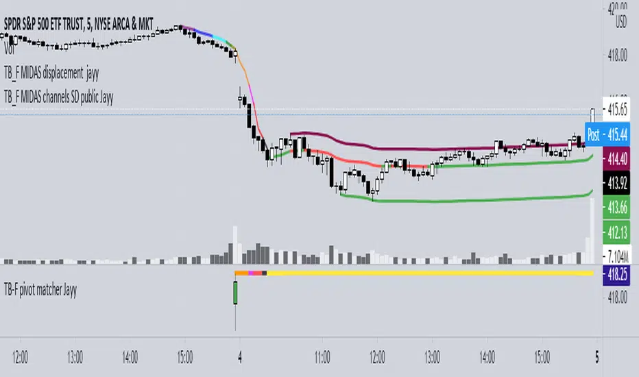
Top Bottom Finder Public version- Jayy This script plots a 6 algos from the Coles/Hawkins "Midas Technical Analysis" book:
Top finder / Bottom Finder (Levine Algo by Bob English)* - onlinelibrary.wiley.com
MIDAS VWAP Gen-1) -
MIDAS VWAP average and deltas
VWAP (Gen-1) using a date or a bar n number can be initiated at bar 0 - useful for a new IPO
Standard Deviation of MIDAS VWAP
MIDAS Displacement Channels (Coles) - edmond.mires.co
An%20Anchored%20VWAP%20Channel%20For%20Congested%20Markets.pdf
* for better results with topfinder and bottomfinder use the companion TB-F Matcher script.
See wiki for a synopsis: en.wikipedia.org
Relevant info can be found in: Midas Technical Analysis: A VWAP Approach to Trading and Investing in Today’s Markets by
Andrew Coles, David G. Hawkins Copyright © 2011 by Andrew Coles and David G. Hawkins.
Appendix C: TradeStation Code for the MIDAS Topfinder/Bottomfinder Curves ported to Tradingview
This script requires a working understanding of "Midas Technical Analysis" Google "Midas Technical Analysis" and a variety of information will appear.
To find fit the curve as described in the Midas book a companion script is required that will after a few manual iterative inputs guide you to the appropriate D value for the for input into this program ( see the TB-F Matcher script). You might also try the Midas average and Deltas as described in the book. I have added the 2nd, 3rd and 4th multiples of Delta.
The advantage is that there is no curve fitting. You still need to select a starting point for Midas or the topfinder bottomfinder (TB_F)
or the VWAP.
////////////////////////////////////////////////////////////////////////////////////////////////////////////////////////////
See the notes in the script below
Cheers Jayy
Volume Range EventsChanges in the feelings (positive, negative, neutral) in the market concerning the valuation of an instrument are often preceded with sudden outbursts of buying and selling frenzies. The aim of this indicator is to report such outbursts. We can see them as expansions of volume, sometimes 10 times more than usual. and as extensions of the trading range, also sometimes 10 times more than usual (e.g. usual range is 10 cent suddenly a whole dollar.) The changes are calculated in such a way that these fit between plus and minus 100 percent, the bars are scaled in some sort of logarithmic way. The Emoline is the same as the one in the True Balance of Power indicator, which I already published
ONLY RISES ARE EVENTS
Sometimes analysts are tempted to give meaning to low volume or small ranges. These simply mean that the market has little interest in trading this instrument. I believe that in such cases the trader needs to wait for expansion and extension events to happen, then he can make a better guess of where the market is heading. As events often mark the beginning or ending of a trend, this indicator provides an early and clear signal, because it doesn’t bother us about non-events.
WHAT IS USUAL?
If the algorithm would use an average as a normal to scale volume or range events, then previous peaks will act as spoilers by making the average so high that a following peak is scaled too small. I developed a function, usual() , that kicks out all extremes of a ‘population of values’ and which returns the average of the non-extreme values. It can be called with any serial. This function is called by both algorithms that report volume and range peaks, which guarantees that the results are really comparable. As this function has a fixed look back of 8 periods, we might state that ‘usual’ is a short lived relative value. I think this doesn’t matter for the practical use of the indicator.
COLORING AND INTERPRETATION
I follow the categories in the ‘Better Volume Indicator’, published by LeazyBear, these are:
1. Climactic Volumes, event >40 % (this means peak is 1.5 X usual)
LIME: Climax Buying Volume, direction up, range event also > 30 %
RED: Climax Selling Volume, direction down, range event also > 30 %
AQUA: Climax Churning Volume, both directions, range event < 30%
2. Smaller Volumes, event <40 %
GREEN: Supportive Volume, both directions, if combined with range event
BLUE: Churning Volume, both directions, if not combined with range event (Professional Trading)
3. Just Range Events
BLACK histogram bars (Amateurish Trading)

BUY & SELL VOLUME TO PRICE PRESSURE by @XeL_ArjonaBUY & SELL PRICE TO VOLUME PRESSURE
By Ricardo M Arjona @XeL_Arjona
DISCLAIMER:
The Following indicator/code IS NOT intended to be a formal investment advice or recommendation by the author, nor should be construed as such. Users will be fully responsible by their use regarding their own trading vehicles/assets.
The embedded code and ideas within this work are FREELY AND PUBLICLY available on the Web for NON LUCRATIVE ACTIVITIES and must remain as is.
Pine Script code MOD's and adaptations by @XeL_Arjona with special mention in regard of:
Buy (Bull) and Sell (Bear) "Power Balance Algorithm" by: Stocks & Commodities V. 21:10 (68-72): "Bull And Bear Balance Indicator by Vadim Gimelfarb"
Normalisation (Filter) from Karthik Marar's VSA work: karthikmarar.blogspot.mx
Buy to Sell Convergence / Divergence and Volume Pressure Counterforce Histogram Ideas by: @XeL_Arjona
WHAT IS THIS?
The following indicators try to acknowledge in a K-I-S-S approach to the eye (Keep-It-Simple-Stupid), the two most important aspects of nearly every trading vehicle: -- PRICE ACTION IN RELATION BY IT'S VOLUME --
Volume Pressure Histogram: Columns plotted in positive are considered the dominant Volume Force for the given period. All "negative" columns represents the counterforce Vol.Press against the dominant.
Buy to Sell Convergence / Divergence: It's a simple adaptation of the popular "Price Percentage Oscillator" or MACD but taking Buying Pressure against Selling Pressure Averages, so given a Positive oscillator reading (>0) represents Bullish dominant Trend and a Negative reading (<0) a Bearish dominant Trend. Histogram is the diff between RAW Volume Pressures Convergence/Divergence minus Normalised ones (Signal) which helps as a confirmation.
Volume bars are by default plotted from RAW Volume Pressure algorithms, but they can be as well filtered with Karthik Marar's approach against a "Total Volume Average" in favor to clean day to day noise like HFT.
ALL NEW IDEAS OR MODIFICATIONS to these indicators are Welcome in favor to deploy a better and more accurate readings. I will be very glad to be notified at Twitter: @XeL_Arjona
Any important addition to this work MUST REMAIN PUBLIC by means of CreativeCommons CC & TradingView. -- 2015