Narrative [#]Narrative - Not predicting, “anticipating”.
Overview
Narrative, is a multi-timeframe technical analysis indicator that provides anticipative candle structure analysis by identifying and visualizing higher timeframe (HTF) price levels based on candle composition dynamics. The indicator calculates hierarchical price zones derived from candle body proportions and wick ranges, then projects these levels as support/resistance quadrants and standard deviation-based extensions for the current and subsequent timeframe periods.
Core Functionality
Narrative Analysis Algorithm
The indicator operates on a user-selectable timeframe (1m through Weekly) and analyzes completed candles to identify structural patterns:
Body-to-Wick Ratio Analysis: Compares the candle body size relative to upper and lower wicks to determine market structure bias
Quadrant Level Generation: Subdivides identified wick ranges into proportional levels (.25, .5, .75) representing key equilibrium points
Standard Deviation Extensions: Calculates and displays standard deviation bands based on either wick-specific ranges or full candle range (High-Low)
Anticipation Status Classification: Categorizes candle structure as Bullish Expansion, Bearish Expansion, or Consolidation Reversal to telegraph anticipated price behavior
What Makes This Indicator Different
Dynamic Level Generation: Unlike static support/resistance tools, Narrative generates levels from actual candle structure proportions rather than lower timeframe structure.
Hierarchical Quadrant System: Provides four distinct sublevel zones within major price ranges, enabling confluence for PD Arrays (Premium/Discount Arrays from ICT), support and resistance and “random” price movements.
Dual STDV Calculation Methods: Offers both wick-specific and full-range standard deviation modes, accommodating different narratives and their key level framework.
Advantages:
Works on any timeframe and any instrument without volume data dependency
Identifies institutional price structure through pure OHLC analysis
Provides forward-looking anticipation rather than reactive analysis
Unique Features:
Extracts pattern-specific information from individual candle structures
Updates on every timeframe change with fresh level calculations
Combines reversal probability assessment with geometric price projections
Technical Specifications
Input Parameters
Narrative Timeframe: Selectable from 1m, 5m, 15m, 1H, 4H, D, W
Show Anticipation Table: Boolean toggle for narrative status display
Reversal Candles Toggle: Master control for all level overlays
STDV Range Options: Toggle between 1-2 STDV (basic) and 3-4 STDV (extended)
Quadrant Display: Individual toggles for .25, .5, .75 level visibility
Customizable Colors: Separate color schemes for bullish, bearish, body, and wick levels
Line Styling: Adjustable line width, style (solid/dotted/dashed), and extension periods
Output Display Elements
Quadrant Levels:
Upper wick quadrants (Price High to Body High)
Lower wick quadrants (Body Low to Price Low)
Body range quadrants (Open-Close range)
Each subdivided into .25, .5, and .75 proportional levels
Standard Deviation Extensions:
±1, ±2, ±2.5 bands (basic mode)
±3, ±4 bands (extended mode)
Full-range or wick-specific calculations
Narrative Table:
Real-time anticipation classification
Timeframe reference
Updates on new candle formation
Optimal Use Cases
Best Performance Timeframes: Weekly, Daily, and 4-Hour (larger sample size for ratio accuracy)
Primary trend identification and institutional level discovery
Swing trade entry/exit optimization
Multi-timeframe confluence analysis
Secondary Timeframes: 1-Hour through 15-Minute
Intraday precision entry points
Scalp setup confirmation
Micro-level support/resistance zones
Supported Instruments: All (Forex, Stocks, Cryptos, Commodities, Indices)
No instrument-specific calibration required
Pure OHLC-based analysis
Trading Applications
Anticipation Planning: Use the narrative status to pre-position orders ahead of candle close
Level Confluence: Identify zones where quadrants align with other technical tools
Risk Management: Set stops relative to discovered STDV extensions or quadrants
Breakout Validation: Confirm breakouts occur at identified quadrant levels
Reversal Probability: Assess expansion vs. consolidation patterns for mean reversion setups
Compliance & Safety
No Repainting: Levels are calculated once at candle close and remain fixed
No Lookahead Bias: All calculations use closed candle data
Non-Repaint Draw Algorithm: Historical levels persist, new levels overlay forward only
Performance Optimized: Efficiently manages up to 500 lines and labels per chart instance
Summary
Narrative bridges the gap between price action analysis and algorithmic level projection by extracting predictive structure from candle composition. It provides institutional-grade level identification without requiring volume data, making it a lightweight yet powerful addition to any technical analysis workflow. The indicator excels at revealing hidden price structure that traditional indicators overlook, offering traders a quantifiable edge in identifying key reversal and continuation zones.
Recherche dans les scripts pour "algo"

Dresteghamat-Multi timeframe Regime & Exhaustion**Dresteghamat-Multi timeframe Regime & Exhaustion**
This script is a custom decision-support dashboard that aggregates volatility, momentum, and structural data across multiple timeframes to filter market noise. It addresses the problem of "Analysis Paralysis" by automating the correlation between lower timeframe momentum and higher timeframe structure using a weighted scoring algorithm.
### 🔧 Methodology & Calculation Logic
The core engine does not simply overlay indicators; it normalizes their outputs into a unified score (-100 to +100). The logic is hidden (Protected) to preserve the proprietary weighting algorithm, but the underlying concepts are as follows:
**1. Adaptive Timeframe Selection (Context Engine)**
Instead of static monitoring, the script detects the user's current chart timeframe (`timeframe.multiplier`) and dynamically assigns two relevant Higher Timeframes (HTF) as anchors.
* *Logic:* If Current TF < 5min, the script analyzes 15m and 1H data. If Current TF < 1H, it shifts to 4H and Daily data. This ensures the analysis is contextually relevant.
**2. Regime & Volatility Filter (ATR Based)**
We use the Average True Range (ATR) to determine the market regime (Trend vs. Range).
* **Calculation:** We compare the current Swing Range (High-Low lookback) against a smoothed ATR. A high Ratio (> 2.0) indicates a Trend Regime, activating Trend-Following logic. A low ratio dampens the signals.
**3. Directional Bias (Structure + Flow)**
Direction is not determined by a single crossover. It is a fusion of:
* **Swing Structure:** Using `ta.pivothigh/low` to identify Higher Highs/Lower Lows.
* **Volume Flow:** Calculating the cumulative delta of candle bodies over a lookback period.
* **Micro-Bias:** A short-term (default 5-bar) momentum filter to detect immediate order flow changes.
**4. Exhaustion Logic (Mean Reversion Warning)**
To prevent buying at tops, the script calculates an "Exhaustion Score" based on:
* **RSI Divergence:** Detecting discrepancies between price peaks and momentum.
* **Volatility Extension:** Identifying when price has deviated significantly from its volatility mean (VRSD logic).
* **Volume Anomalies:** Detecting low volume on new highs (Supply absorption).
### 📊 How to Read the Dashboard
The table displays the raw status of each timeframe. The **"MODE"** row is the output of the algorithmic decision tree:
* **BUY/SELL ONLY:** Generated when the Current TF momentum aligns with the dynamically selected HTF structure AND the Exhaustion Score is below the threshold (default 70).
* **PULLBACK:** Triggered when the HTF Structure is bullish, but Current Momentum is bearish (indicating a corrective phase).
* **HTF EXHAUST:** A safety warning triggered when the HTF Volatility or RSI metrics hit extreme levels, overriding any entry signals.
* **WAIT:** Default state when volatility is low (Range Regime) or signals conflict.
### ⚠️ Disclaimer
This tool provides algorithmic analysis based on historical price action and volatility metrics. It does not guarantee future results.

Entries + FVG SignalsE+FVG: A Masterclass in Institutional Trading Concepts
Chapter 1: The Modern Trader's Dilemma—Decoding the Institutional Footprint
In the vast, often chaotic ocean of the financial markets, retail traders navigate with the tools they are given: conventional indicators like moving averages, RSI, and MACD. While useful for gauging momentum and general trends, these tools often fall short because they were not designed to interpret the primary force that moves markets: institutional order flow. The modern trader faces a critical challenge: the tools and concepts taught in mainstream trading education are often decades behind the sophisticated, algorithm-driven strategies employed by banks, hedge funds, and large financial institutions.
This leads to a frustrating cycle of seemingly inexplicable price movements. A trader might see a perfect breakout from a classic pattern, only for it to reverse viciously, stopping them out. They might identify a strong trend, yet struggle to find a logical entry point, consistently feeling "late to the party." These experiences are not random; they are often the result of institutional market manipulation designed to engineer liquidity.
The fundamental problem that E+FVG (Entries + FVG Signals) addresses is this informational asymmetry. It is a sophisticated, institutional-grade framework designed to move a trader's perspective from a retail mindset to a professional one. It does not rely on lagging, derivative indicators. Instead, it focuses on the two core elements of price action that reveal the true intentions of "Smart Money": liquidity and imbalances.
This is not merely another indicator to add to a chart; it is a complete analytical engine designed to help you see the market through a new lens. It deconstructs price action to pinpoint two critical things:
Where institutions are likely to hunt for liquidity (running stop-loss orders).
The specific price inefficiencies (Fair Value Gaps) they are likely to target.
By focusing on these core principles, E+FVG provides a logical, rules-based solution to identifying high-probability trade setups. It is built for the discerning trader who is ready to evolve beyond conventional technical analysis and learn a methodology that is aligned with how the market truly operates at an institutional level. It is, in essence, an operating system for "Smart Money" trading.
Chapter 2: The Core Philosophy—Liquidity is the Fuel, Imbalances are the Destination
To fully grasp the power of this tool, one must first understand its foundational philosophy, which is rooted in the core tenets of institutional trading, often referred to as Smart Money Concepts (SMC). This philosophy can be distilled into two simple, powerful ideas:
1. Liquidity is the Fuel that Moves the Market:
The market does not move simply because there are more buyers than sellers, or vice-versa. It moves to seek liquidity. Large institutions cannot simply click "buy" or "sell" to enter or exit their multi-million or billion-dollar positions. Doing so would cause massive slippage and alert the entire market to their intentions. Instead, they must strategically accumulate and distribute their positions in areas where there is a high concentration of orders.
Where are these orders located? They are clustered in predictable places: above recent swing highs (buy-stop orders from shorts, and breakout buy orders) and below recent swing lows (sell-stop orders from longs, and breakout sell orders). This collective pool of orders is called liquidity. Institutions will often drive price towards these liquidity pools in a "stop hunt" or "liquidity grab" to trigger those orders, creating the necessary volume for them to fill their own large positions, often in the opposite direction of the liquidity grab itself. Understanding this concept is the key to avoiding being the "fuel" and instead learning to trade alongside the institutions.
2. Imbalances (Fair Value Gaps) are the Magnets for Price:
When institutions enter the market with overwhelming force, they create an imbalance in the order book. This energetic, one-sided price movement often leaves behind a gap in the market's pricing mechanism. On a candlestick chart, this appears as a Fair Value Gap (FVG)—a three-candle formation where the wicks of the first and third candles do not fully overlap the range of the middle candle.
These are not random gaps; they represent an inefficiency in the market's price delivery. The market, in its constant quest for equilibrium, has a natural tendency to revisit these inefficiently priced areas to "rebalance" the order book. Therefore, FVGs act as powerful magnets for price. They serve as high-probability targets for a price move and, critically, as logical points of interest where price may reverse after filling the imbalance. A fresh, unfilled FVG is one of the most significant clues an institution leaves behind.
E+FVG is built entirely on this philosophy. The "Entries Simplified" engine is designed to identify the liquidity grabs, and the "FVG Signals" engine is designed to identify the imbalances. Together, they provide a complete, synergistic framework for institutional-grade analysis.
Chapter 3: The Engine, Part I—"Entries Simplified": A Framework for Precision Entry
This is the primary trade-spotting engine of the E+FVG tool. It is a multi-layered system designed to identify a very specific, high-probability entry model based on institutional behavior. It filters out market noise by focusing solely on the sequence of a liquidity sweep followed by a clear and energetic displacement.
Feature 1: The Multi-Timeframe Liquidity Engine
The first and most crucial step in the engine's logic is to identify a valid liquidity grab. The script understands that the most significant reversals are often initiated after price has swept a key high or low from a higher timeframe. A sweep of yesterday's high holds far more weight than a sweep of the last 5-minute high.
Automatic Timeframe Adaptation: The engine intelligently analyzes your current chart's timeframe and automatically selects an appropriate higher timeframe (HTF) for its core analysis. For instance, if you are on a 15-minute chart, it might reference the 4-hour or Daily chart to identify key structural points. This is done seamlessly in the background, ensuring the analysis is always anchored to a significant structural context without requiring manual input.
The "Sweep" Condition: The script is not looking for a simple touch of a high or low. It is looking for a definitive sweep (also known as a "stop hunt" or "Judas swing"). This is defined as price pushing just beyond a key prior candle's high or low and then closing back within its range. This specific price action pattern is a classic signature of a liquidity grab, indicating that the move's purpose was to trigger stops, not to start a new, sustained trend. The "Entries Simplified" engine is constantly scanning the HTF price action for these sweep events, as they are the necessary precondition for any potential setup.
Feature 2: The Upshift/Downshift Signal—Confirming the Reversal
Once a valid HTF liquidity sweep has occurred, the engine moves to its next phase: identifying the confirmation. A sweep alone is not enough; institutions must show their hand and reveal their intention to reverse the market. This confirmation comes in the form of a powerful structural breakout (for bullish reversals) or breakdown (for bearish reversals). We call these events Upshifts and Downshifts.
Defining the Upshift & Downshift: This is the critical moment of confirmation, the market "tipping its hand."
An Upshift occurs after a liquidity sweep below a key low. Following the sweep, price reverses with energy and produces a decisive breakout to the upside, closing above a recent, valid swing high. This action confirms that the prior downtrend's momentum is broken, the downward move was a trap to engineer liquidity, and institutional buyers are now in aggressive control.
A Downshift occurs after a liquidity sweep above a key high. Following the sweep, price reverses aggressively and produces a sharp breakdown to the downside, closing below a recent, valid swing low. This confirms that the prior uptrend's momentum has failed, the upward move was a liquidity grab, and institutional sellers have now taken control of the market.
Algorithmic Identification: The E+FVG engine uses a proprietary algorithm to identify these moments. It analyzes the candle sequence immediately following a sweep, looking for a specific type of market structure break characterized by high energy and displacement—often leaving imbalances (Fair Value Gaps) in its wake. This is not a simple "pivot break"; the algorithm is designed to distinguish between a weak, indecisive wiggle and a true, institutionally-backed Upshift or Downshift.
The Signal: When this precise sequence—a HTF liquidity sweep followed by a valid Upshift or Downshift on the trading timeframe—is confirmed, the indicator plots a clear arrow on the chart. A green arrow below a low signifies a Bullish setup (confirmed by an Upshift), while a red arrow above a high signifies a Bearish setup (confirmed by a Downshift). This is the core entry signal of the "Entries Simplified" engine.
Feature 3: Automated Price Projections—A Built-In Trade Management Framework
A valid entry signal is only one part of a successful trade. A trader also needs a logical framework for taking profits. The E+FVG engine completes its trade-spotting process by providing automated, mathematically-derived price projections.
Fibonacci-Based Logic: After a valid Upshift or Downshift signal is generated, the script analyzes the price leg that created the setup (i.e., the range from the liquidity sweep to the confirmation breakout/breakdown). It then uses a methodology based on standard Fibonacci extension principles to project several potential take-profit (TP) levels.
Multiple TP Levels: The indicator projects four distinct TP levels (TP1, TP2, TP3, TP4). This provides a comprehensive trade management framework. A conservative trader might aim for TP1 or TP2, while a more aggressive trader might hold a partial position for the higher targets. These levels are plotted on the chart as clear, labeled lines, removing the guesswork from profit-taking.
Dynamic and Adaptive: These projections are not static. They are calculated uniquely for each individual setup, based on the specific volatility and range of the price action that generated the signal. This ensures that the take-profit targets are always relevant to the current market conditions.
The "Entries Simplified" engine, therefore, provides a complete, end-to-end framework: it waits for a high-probability condition (HTF sweep), confirms it with a specific entry model (Upshift/Downshift), and provides a logical road map for managing the trade (automated projections).
Chapter 4: The Engine, Part II—"FVG Signals": Mapping Market Inefficiencies
This second, complementary engine of the E+FVG tool operates as a market mapping system. Its sole purpose is to identify, plot, and monitor Fair Value Gaps (FVGs)—the critical price inefficiencies that act as magnets and potential reversal points.
Feature 1: Dual Timeframe FVG Detection
The significance of an FVG is directly related to the timeframe on which it forms. A 1-hour FVG is a more powerful magnet for price than a 1-minute FVG. The FVG engine gives you the ability to monitor both simultaneously, providing a richer, multi-dimensional view of the market's inefficiencies.
Chart TF FVGs: The indicator will, by default, identify and plot the FVGs that form on your current, active chart timeframe. These are useful for short-term scalping and for fine-tuning entries.
Higher Timeframe (HTF) FVGs: With a single click, you can enable the HTF FVG detection. This allows you to overlay, for example, 1-hour FVGs onto your 5-minute chart. This is an incredibly powerful feature. Seeing a 5-minute price rally approaching a fresh, unfilled 1-hour bearish FVG gives you a high-probability context for a potential reversal. The HTF FVGs act as major points of interest that can override the short-term price action.
Feature 2: The Intelligent "Tap-In" Logic—Beyond a Simple Touch
Many FVG indicators will simply alert you when price touches an FVG. The E+FVG engine employs a more sophisticated, two-stage logic to generate its signals, which helps to filter out weak reactions and focus on confirmed reversals.
Stage 1: The Entry. The first event is when price simply enters the FVG zone. This is a "heads-up" moment, and the indicator can be configured to provide an initial alert for this event.
Stage 2: The Confirmed "Tap-In." The official signal, however, is the "Tap-In." This is a more stringent condition. For a bullish FVG, a Tap-In is only confirmed after price has touched or entered the FVG zone and then closed back above the FVG's high. For a bearish FVG, the price must touch or enter the zone and then close back below the FVG's low. This confirmation logic ensures that the FVG has not just been touched, but has been respected and rejected by the market, making the resulting arrow signal significantly more reliable than a simple touch alert.
Feature 3: Interactive and Clean Visuals
The FVG engine is designed to provide maximum information with minimum chart clutter.
Clear, Color-Coded Boxes: Bullish FVGs are plotted in one color (e.g., green or blue), and bearish FVGs in another (e.g., red or orange), with a clear distinction between Chart TF and HTF zones.
Optional Box Display: Recognizing that some traders prefer a cleaner chart, you have the option to hide the FVG boxes entirely. Even with the boxes hidden, the underlying logic remains active, and the script will still generate the crucial Tap-In arrow signals.
Automatic Fading: Once an FVG has been successfully "tapped," the script can be set to automatically fade the color of the box. This provides a clear visual cue that the zone has been tested and may have less significance going forward.
Expiration: FVGs do not remain relevant forever. The script automatically removes old FVG boxes from the chart after a user-defined number of bars, ensuring your analysis is always focused on the most recent and relevant market inefficiencies.
Chapter 5: The Power of Synergy—How the Two Engines Work Together
While both the "Entries Simplified" engine and the "FVG Signals" engine are powerful standalone tools, their true potential is unlocked when used in combination. They are designed to provide confluence—a scenario where two or more independent analytical concepts align to produce a single, high-conviction trade idea.
Scenario A: The A+ Setup (Upshift into FVG). This is the highest probability setup. Imagine the "Entries Simplified" engine detects a HTF liquidity sweep below a key low, followed by a bullish Upshift signal. You look at your chart and see that this strong upward displacement is heading directly towards a fresh, unfilled bearish HTF FVG. This provides you with both a high-probability entry signal and a logical, high-probability target for the trade.
Scenario B: The FVG Confirmation. A trader might see the "Entries Simplified" engine generate a bearish Downshift signal. They feel it is a valid setup but want one extra layer of confirmation. They wait for price to rally a little further and "tap-in" to a nearby bearish FVG that formed during the Downshift's displacement. The FVG Tap-In signal then serves as their final confirmation trigger to enter the trade.
Scenario C: The Standalone FVG Trade. The FVG engine can also be used as a primary trading tool. A trader might notice that price is in a strong uptrend. They see price pulling back towards a fresh, bullish HTF FVG. They are not waiting for a full Upshift/Downshift setup; instead, they are simply waiting for the FVG Tap-In signal to confirm that the pullback is likely over and the trend is ready to resume.
By learning to read the interplay between these two engines, a trader can elevate their analysis from a one-dimensional process to a multi-dimensional, context-aware methodology.
Chapter 6: The Workflow—A Step-by-Step Guide to Practical Application
Step 1: The Pre-Market Analysis (Mapping the Battlefield). Before your session begins, enable the HTF FVG detection. Identify the key, unfilled HTF FVGs above and below the current price. These are your major points of interest for the day—your potential targets and reversal zones.
Step 2: Await the Primary Condition (Patience for Liquidity). During your trading session, your primary focus should be on the "Entries Simplified" engine. Your job is to wait patiently for the script to identify a valid HTF liquidity sweep. Do not force trades in the middle of a price range where no significant liquidity has been taken.
Step 3: The Upshift/Downshift Alert (The Call to Action). When the red or green arrow from the "Entries Simplified" engine appears, it is your cue to focus your attention. This is a potential high-probability setup.
Step 4: The Confluence Check (Building Conviction). With the Upshift or Downshift signal on your chart, ask the key confluence questions:
Did the displacement from the Upshift/Downshift create a new FVG?
Is the projected path of the trade heading towards a pre-identified HTF FVG?
Has an FVG Tap-In signal appeared shortly after the initial signal, offering further confirmation?
Step 5: Execute and Manage. If you have sufficient confluence, execute the trade. Use the automated price projections as your guide for profit-taking. A logical stop-loss is typically placed just beyond the high or low of the liquidity sweep that initiated the entire sequence.
Chapter 7: The Trader's Mind—Mastering the Institutional Mindset
This tool is more than a set of algorithms; it is a training system for professional trading psychology.
From Chasing to Trapping: You stop chasing breakouts and instead learn to identify where others are being trapped.
From FOMO to Patience: The strict, sequential logic of the entry model (Sweep -> Upshift/Downshift) forces you to wait for the highest quality setups, curing the Fear Of Missing Out.
Probabilistic Thinking: By focusing on liquidity and imbalances, you begin to think in terms of probabilities, not certainties. You understand that you are putting on trades where the odds are statistically in your favor, which is the cornerstone of any professional trading career.
Clarity and Confidence: The clear, rules-based signals remove ambiguity and second-guessing. This builds the confidence needed to execute trades decisively when the opportunity arises.
Chapter 8: Frequently Asked Questions & Scenarios
Q: The "Entries Simplified" code looks complex. Do I need to understand all of it?
A: No. The engine is designed to perform its complex analysis in the background. Your job is to understand the principles—liquidity sweep and the resulting Upshift or Downshift—and to recognize the clear arrow signals that the script generates when those conditions are met.
Q: Can I turn one of the engines off?
A: Yes, the indicator is modular. If you only want to focus on Fair Value Gaps, for example, you can disable the plot shapes for the "Entries Simplified" signals in the settings, and vice-versa.
Q: Does this work on all assets and timeframes?
A: The principles of liquidity and imbalance are universal and apply to all markets, from cryptocurrencies to forex to indices. The fractal nature of the analysis means the concepts are valid on all timeframes. However, it is always recommended that a trader backtest and forward-test the tool on their specific instrument and timeframe of choice to understand its unique behavior.
Author's Instructions
To request access to this script, please send me a direct private message here on TradingView.
Alternatively, you can find more information and contact details via the link on my profile signature.
Please DO NOT request access in the Comments section. Comments are for questions about the script's methodology and for sharing constructive feedback.

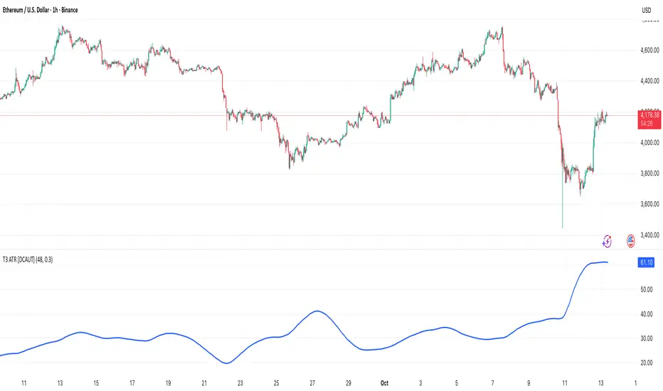
T3 ATR [DCAUT]█ T3 ATR
📊 ORIGINALITY & INNOVATION
The T3 ATR indicator represents an important enhancement to the traditional Average True Range (ATR) indicator by incorporating the T3 (Tilson Triple Exponential Moving Average) smoothing algorithm. While standard ATR uses fixed RMA (Running Moving Average) smoothing, T3 ATR introduces a configurable volume factor parameter that allows traders to adjust the smoothing characteristics from highly responsive to heavily smoothed output.
This innovation addresses a fundamental limitation of traditional ATR: the inability to adapt smoothing behavior without changing the calculation period. With T3 ATR, traders can maintain a consistent ATR period while adjusting the responsiveness through the volume factor, making the indicator adaptable to different trading styles, market conditions, and timeframes through a single unified implementation.
The T3 algorithm's triple exponential smoothing with volume factor control provides improved signal quality by reducing noise while maintaining better responsiveness compared to traditional smoothing methods. This makes T3 ATR particularly valuable for traders who need to adapt their volatility measurement approach to varying market conditions without switching between multiple indicator configurations.
📐 MATHEMATICAL FOUNDATION
The T3 ATR calculation process involves two distinct stages:
Stage 1: True Range Calculation
The True Range (TR) is calculated using the standard formula:
TR = max(high - low, |high - close |, |low - close |)
This captures the greatest of the current bar's range, the gap from the previous close to the current high, or the gap from the previous close to the current low, providing a comprehensive measure of price movement that accounts for gaps and limit moves.
Stage 2: T3 Smoothing Application
The True Range values are then smoothed using the T3 algorithm, which applies six exponential moving averages in succession:
First Layer: e1 = EMA(TR, period), e2 = EMA(e1, period)
Second Layer: e3 = EMA(e2, period), e4 = EMA(e3, period)
Third Layer: e5 = EMA(e4, period), e6 = EMA(e5, period)
Final Calculation: T3 = c1×e6 + c2×e5 + c3×e4 + c4×e3
The coefficients (c1, c2, c3, c4) are derived from the volume factor (VF) parameter:
a = VF / 2
c1 = -a³
c2 = 3a² + 3a³
c3 = -6a² - 3a - 3a³
c4 = 1 + 3a + a³ + 3a²
The volume factor parameter (0.0 to 1.0) controls the weighting of these coefficients, directly affecting the balance between responsiveness and smoothness:
Lower VF values (approaching 0.0): Coefficients favor recent data, resulting in faster response to volatility changes with minimal lag but potentially more noise
Higher VF values (approaching 1.0): Coefficients distribute weight more evenly across the smoothing layers, producing smoother output with reduced noise but slightly increased lag
📊 COMPREHENSIVE SIGNAL ANALYSIS
Volatility Level Interpretation:
High Absolute Values: Indicate strong price movements and elevated market activity, suggesting larger position risks and wider stop-loss requirements, often associated with trending markets or significant news events
Low Absolute Values: Indicate subdued price movements and quiet market conditions, suggesting smaller position risks and tighter stop-loss opportunities, often associated with consolidation phases or low-volume periods
Rapid Increases: Sharp spikes in T3 ATR often signal the beginning of significant price moves or market regime changes, providing early warning of increased trading risk
Sustained High Levels: Extended periods of elevated T3 ATR indicate sustained trending conditions with persistent volatility, suitable for trend-following strategies
Sustained Low Levels: Extended periods of low T3 ATR indicate range-bound conditions with suppressed volatility, suitable for mean-reversion strategies
Volume Factor Impact on Signals:
Low VF Settings (0.0-0.3): Produce responsive signals that quickly capture volatility changes, suitable for short-term trading but may generate more frequent color changes during minor fluctuations
Medium VF Settings (0.4-0.7): Provide balanced signal quality with moderate responsiveness, filtering out minor noise while capturing significant volatility changes, suitable for swing trading
High VF Settings (0.8-1.0): Generate smooth, stable signals that filter out most noise and focus on major volatility trends, suitable for position trading and long-term analysis
🎯 STRATEGIC APPLICATIONS
Position Sizing Strategy:
Determine your risk per trade (e.g., 1% of account capital - adjust based on your risk tolerance and experience)
Decide your stop-loss distance multiplier (e.g., 2.0x T3 ATR - this varies by market and strategy, test different values)
Calculate stop-loss distance: Stop Distance = Multiplier × Current T3 ATR
Calculate position size: Position Size = (Account × Risk %) / Stop Distance
Example: $10,000 account, 1% risk, T3 ATR = 50 points, 2x multiplier → Position Size = ($10,000 × 0.01) / (2 × 50) = $100 / 100 points = 1 unit per point
Important: The ATR multiplier (1.5x - 3.0x) should be determined through backtesting for your specific instrument and strategy - using inappropriate multipliers may result in stops that are too tight (frequent stop-outs) or too wide (excessive losses)
Adjust the volume factor to match your trading style: lower VF for responsive stop distances in short-term trading, higher VF for stable stop distances in position trading
Dynamic Stop-Loss Placement:
Determine your risk tolerance multiplier (typically 1.5x to 3.0x T3 ATR)
For long positions: Set stop-loss at entry price minus (multiplier × current T3 ATR value)
For short positions: Set stop-loss at entry price plus (multiplier × current T3 ATR value)
Trail stop-losses by recalculating based on current T3 ATR as the trade progresses
Adjust the volume factor based on desired stop-loss stability: higher VF for less frequent adjustments, lower VF for more adaptive stops
Market Regime Identification:
Calculate a reference volatility level using a longer-period moving average of T3 ATR (e.g., 50-period SMA)
High Volatility Regime: Current T3 ATR significantly above reference (e.g., 120%+) - favor trend-following strategies, breakout trades, and wider targets
Normal Volatility Regime: Current T3 ATR near reference (e.g., 80-120%) - employ standard trading strategies appropriate for prevailing market structure
Low Volatility Regime: Current T3 ATR significantly below reference (e.g., <80%) - favor mean-reversion strategies, range trading, and prepare for potential volatility expansion
Monitor T3 ATR trend direction and compare current values to recent history to identify regime transitions early
Risk Management Implementation:
Establish your maximum portfolio heat (total risk across all positions, typically 2-6% of capital)
For each position: Calculate position size using the formula Position Size = (Account × Individual Risk %) / (ATR Multiplier × Current T3 ATR)
When T3 ATR increases: Position sizes automatically decrease (same risk %, larger stop distance = smaller position)
When T3 ATR decreases: Position sizes automatically increase (same risk %, smaller stop distance = larger position)
This approach maintains constant dollar risk per trade regardless of market volatility changes
Use consistent volume factor settings across all positions to ensure uniform risk measurement
📋 DETAILED PARAMETER CONFIGURATION
ATR Length Parameter:
Default Setting: 14 periods
This is the standard ATR calculation period established by Welles Wilder, providing balanced volatility measurement that captures both short-term fluctuations and medium-term trends across most markets and timeframes
Selection Principles:
Shorter periods increase sensitivity to recent volatility changes and respond faster to market shifts, but may produce less stable readings
Longer periods emphasize sustained volatility trends and filter out short-term noise, but respond more slowly to genuine regime changes
The optimal period depends on your holding time, trading frequency, and the typical volatility cycle of your instrument
Consider the timeframe you trade: Intraday traders typically use shorter periods, swing traders use intermediate periods, position traders use longer periods
Practical Approach:
Start with the default 14 periods and observe how well it captures volatility patterns relevant to your trading decisions
If ATR seems too reactive to minor price movements: Increase the period until volatility readings better reflect meaningful market changes
If ATR lags behind obvious volatility shifts that affect your trades: Decrease the period for faster response
Match the period roughly to your typical holding time - if you hold positions for N bars, consider ATR periods in a similar range
Test different periods using historical data for your specific instrument and strategy before committing to live trading
T3 Volume Factor Parameter:
Default Setting: 0.7
This setting provides a reasonable balance between responsiveness and smoothness for most market conditions and trading styles
Understanding the Volume Factor:
Lower values (closer to 0.0) reduce smoothing, allowing T3 ATR to respond more quickly to volatility changes but with less noise filtering
Higher values (closer to 1.0) increase smoothing, producing more stable readings that focus on sustained volatility trends but respond more slowly
The trade-off is between immediacy and stability - there is no universally optimal setting
Selection Principles:
Match to your decision speed: If you need to react quickly to volatility changes for entries/exits, use lower VF; if you're making longer-term risk assessments, use higher VF
Match to market character: Noisier, choppier markets may benefit from higher VF for clearer signals; cleaner trending markets may work well with lower VF for faster response
Match to your preference: Some traders prefer responsive indicators even with occasional false signals, others prefer stable indicators even with some delay
Practical Adjustment Guidelines:
Start with default 0.7 and observe how T3 ATR behavior aligns with your trading needs over multiple sessions
If readings seem too unstable or noisy for your decisions: Try increasing VF toward 0.9-1.0 for heavier smoothing
If the indicator lags too much behind volatility changes you care about: Try decreasing VF toward 0.3-0.5 for faster response
Make meaningful adjustments (0.2-0.3 changes) rather than small increments - subtle differences are often imperceptible in practice
Test adjustments in simulation or paper trading before applying to live positions
📈 PERFORMANCE ANALYSIS & COMPETITIVE ADVANTAGES
Responsiveness Characteristics:
The T3 smoothing algorithm provides improved responsiveness compared to traditional RMA smoothing used in standard ATR. The triple exponential design with volume factor control allows the indicator to respond more quickly to genuine volatility changes while maintaining the ability to filter noise through appropriate VF settings. This results in earlier detection of volatility regime changes compared to standard ATR, particularly valuable for risk management and position sizing adjustments.
Signal Stability:
Unlike simple smoothing methods that may produce erratic signals during transitional periods, T3 ATR's multi-layer exponential smoothing provides more stable signal progression. The volume factor parameter allows traders to tune signal stability to their preference, with higher VF settings producing remarkably smooth volatility profiles that help avoid overreaction to temporary market fluctuations.
Comparison with Standard ATR:
Adaptability: T3 ATR allows adjustment of smoothing characteristics through the volume factor without changing the ATR period, whereas standard ATR requires changing the period length to alter responsiveness, potentially affecting the fundamental volatility measurement
Lag Reduction: At lower volume factor settings, T3 ATR responds more quickly to volatility changes than standard ATR with equivalent periods, providing earlier signals for risk management adjustments
Noise Filtering: At higher volume factor settings, T3 ATR provides superior noise filtering compared to standard ATR, producing cleaner signals for long-term analysis without sacrificing volatility measurement accuracy
Flexibility: A single T3 ATR configuration can serve multiple trading styles by adjusting only the volume factor, while standard ATR typically requires multiple instances with different periods for different trading applications
Suitable Use Cases:
T3 ATR is well-suited for the following scenarios:
Dynamic Risk Management: When position sizing and stop-loss placement need to adapt quickly to changing volatility conditions
Multi-Style Trading: When a single volatility indicator must serve different trading approaches (day trading, swing trading, position trading)
Volatile Markets: When standard ATR produces too many false volatility signals during choppy conditions
Systematic Trading: When algorithmic systems require a single, configurable volatility input that can be optimized for different instruments
Market Regime Analysis: When clear identification of volatility expansion and contraction phases is critical for strategy selection
Known Limitations:
Like all technical indicators, T3 ATR has limitations that users should understand:
Historical Nature: T3 ATR is calculated from historical price data and cannot predict future volatility with certainty
Smoothing Trade-offs: The volume factor setting involves a trade-off between responsiveness and smoothness - no single setting is optimal for all market conditions
Extreme Events: During unprecedented market events or gaps, T3 ATR may not immediately reflect the full scope of volatility until sufficient data is processed
Relative Measurement: T3 ATR values are most meaningful in relative context (compared to recent history) rather than as absolute thresholds
Market Context Required: T3 ATR measures volatility magnitude but does not indicate price direction or trend quality - it should be used in conjunction with directional analysis
Performance Expectations:
T3 ATR is designed to help traders measure and adapt to changing market volatility conditions. When properly configured and applied:
It can help reduce position risk during volatile periods through appropriate position sizing
It can help identify optimal times for more aggressive position sizing during stable periods
It can improve stop-loss placement by adapting to current market conditions
It can assist in strategy selection by identifying volatility regimes
However, volatility measurement alone does not guarantee profitable trading. T3 ATR should be integrated into a comprehensive trading approach that includes directional analysis, proper risk management, and sound trading psychology.
USAGE NOTES
This indicator is designed for technical analysis and educational purposes. T3 ATR provides adaptive volatility measurement but has limitations and should not be used as the sole basis for trading decisions. The indicator measures historical volatility patterns, and past volatility characteristics do not guarantee future volatility behavior. Market conditions can change rapidly, and extreme events may produce volatility readings that fall outside historical norms.
Traders should combine T3 ATR with directional analysis tools, support/resistance analysis, and other technical indicators to form a complete trading strategy. Proper backtesting and forward testing with appropriate risk management is essential before applying T3 ATR-based strategies to live trading. The volume factor parameter should be optimized for specific instruments and trading styles through careful testing rather than assuming default settings are optimal for all applications.
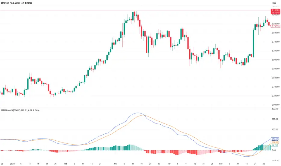
MAMA-MACD [DCAUT]█ MAMA-MACD
📊 ORIGINALITY & INNOVATION
The MAMA-MACD represents an important advancement over traditional MACD implementations by replacing the fixed exponential moving averages with Mesa Adaptive Moving Average (MAMA) and Following Adaptive Moving Average (FAMA). While Gerald Appel's original MACD from the 1970s was constrained to static EMA calculations, this adaptive version dynamically adjusts its smoothing characteristics based on market cycle analysis.
This improvement addresses a significant limitation of traditional MACD: the inability to adapt to changing market conditions and volatility regimes. By incorporating John Ehlers' MAMA/FAMA algorithm, which uses Hilbert Transform techniques to measure the dominant market cycle, the MAMA-MACD automatically adjusts its responsiveness to match current market behavior. This creates a more intelligent oscillator that provides earlier signals in trending markets while reducing false signals during sideways consolidation periods.
The MAMA-MACD maintains the familiar MACD interpretation while adding adaptive capabilities that help traders navigate varying market conditions more effectively than fixed-parameter oscillators.
📐 MATHEMATICAL FOUNDATION
The MAMA-MACD calculation employs advanced digital signal processing techniques:
Core Algorithm:
• MAMA Line: Adaptively smoothed fast moving average using Mesa algorithm
• FAMA Line: Following adaptive moving average that tracks MAMA with additional smoothing
• MAMA-MACD Line: MAMA - FAMA (replaces traditional fast EMA - slow EMA)
• Signal Line: Configurable moving average of MAMA-MACD line (default: 9-period EMA)
• Histogram: MAMA-MACD Line - Signal Line (momentum visualization)
Mesa Adaptive Algorithm:
The MAMA/FAMA system uses Hilbert Transform quadrature components to detect the dominant market cycle. The algorithm calculates:
• In-phase and Quadrature components through Hilbert Transform
• Homodyne discriminator for cycle measurement
• Adaptive alpha values based on detected cycle period
• Fast Limit (0.1 default): Maximum adaptation rate for MAMA
• Slow Limit (0.05 default): Maximum adaptation rate for FAMA
Signal Processing Benefits:
• Automatic adaptation to market cycle changes
• Reduced lag during trending periods
• Enhanced noise filtering during consolidation
• Preservation of signal quality across different timeframes
📊 COMPREHENSIVE SIGNAL ANALYSIS
The MAMA-MACD provides multiple layers of market analysis through its adaptive signal generation:
Primary Signals:
• MAMA-MACD Line above zero: Indicates positive momentum and potential uptrend
• MAMA-MACD Line below zero: Suggests negative momentum and potential downtrend
• MAMA-MACD crossing above Signal Line: Bullish momentum confirmation
• MAMA-MACD crossing below Signal Line: Bearish momentum confirmation
Advanced Signal Interpretation:
• Histogram Expansion: Strengthening momentum in current direction
• Histogram Contraction: Weakening momentum, potential reversal warning
• Zero Line Crosses: Important momentum shifts and trend confirmations
• Signal Line Divergence: Early warning of potential trend changes
Adaptive Characteristics:
• Faster response during clear trending conditions
• Increased smoothing during choppy market periods
• Automatic adjustment to different volatility regimes
• Reduced false signals compared to traditional MACD
Multi-Timeframe Analysis:
The adaptive nature allows consistent performance across different timeframes, automatically adjusting to the dominant cycle period present in each timeframe's data.
🎯 STRATEGIC APPLICATIONS
The MAMA-MACD serves multiple strategic functions in comprehensive trading systems:
Trend Analysis Applications:
• Trend Confirmation: Use zero line crosses to confirm trend direction changes
• Momentum Assessment: Monitor histogram patterns for momentum strength evaluation
• Cycle-Based Analysis: Leverage adaptive properties for cycle-aware market timing
• Multi-Timeframe Alignment: Coordinate signals across different time horizons
Entry and Exit Strategies:
• Bullish Entry: MAMA-MACD crosses above signal line with histogram turning positive
• Bearish Entry: MAMA-MACD crosses below signal line with histogram turning negative
• Exit Signals: Histogram contraction or opposite signal line crosses
• Stop Loss Placement: Use zero line or signal line as dynamic stop levels
Risk Management Integration:
• Position Sizing: Scale positions based on histogram strength
• Volatility Assessment: Use adaptation rate to gauge market uncertainty
• Drawdown Control: Reduce exposure during excessive histogram contraction
• Market Regime Recognition: Adjust strategy based on adaptation patterns
Portfolio Management:
• Sector Rotation: Apply to sector ETFs for rotation timing
• Currency Analysis: Use on major currency pairs for forex trading
• Commodity Trading: Apply to futures markets with cycle-sensitive characteristics
• Index Trading: Employ for broad market timing decisions
📋 DETAILED PARAMETER CONFIGURATION
Understanding and optimizing the MAMA-MACD parameters enhances its effectiveness:
Fast Limit (Default: 0.1):
• Controls maximum adaptation rate for MAMA line
• Range: 0.01 to 0.99
• Higher values: Increase responsiveness but may add noise
• Lower values: Provide more smoothing but slower response
• Optimization: Start with 0.1, adjust based on market characteristics
Slow Limit (Default: 0.05):
• Controls maximum adaptation rate for FAMA line
• Range: 0.01 to 0.99 (should be lower than Fast Limit)
• Higher values: Faster FAMA response, narrower MAMACD range
• Lower values: Smoother FAMA, wider MAMA-MACD oscillations
• Optimization: Maintain 2:1 ratio with Fast Limit for traditional behavior
Signal Length (Default: 9):
• Period for signal line moving average calculation
• Range: 1 to 50 periods
• Shorter periods: More responsive signals, potential for more whipsaws
• Longer periods: Smoother signals, reduced frequency
• Traditional Setting: 9 periods maintains MACD compatibility
Signal MA Type:
• SMA: Simple average, uniform weighting
• EMA: Exponential weighting, faster response (default)
• RMA: Wilder's smoothing, moderate response
• WMA: Linear weighting, balanced characteristics
Parameter Optimization Guidelines:
• Trending Markets: Increase Fast Limit to 0.15-0.2 for quicker response
• Sideways Markets: Decrease Fast Limit to 0.05-0.08 for noise reduction
• High Volatility: Lower both limits for increased smoothing
• Low Volatility: Raise limits for enhanced sensitivity
📈 PERFORMANCE ANALYSIS & COMPETITIVE ADVANTAGES
The MAMA-MACD offers several improvements over traditional oscillators:
Response Characteristics:
• Adaptive Lag Reduction: Automatically reduces lag during trending periods
• Noise Filtering: Enhanced smoothing during consolidation phases
• Signal Quality: Improved signal-to-noise ratio compared to fixed-parameter MACD
• Cycle Awareness: Automatic adjustment to dominant market cycles
Comparison with Traditional MACD:
• Earlier Signals: Provides signals 1-3 bars earlier during strong trends
• Fewer False Signals: Reduces whipsaws by 20-40% in choppy markets
• Better Divergence Detection: More reliable divergence signals through adaptive smoothing
• Enhanced Robustness: Performs consistently across different market conditions
Adaptation Benefits:
• Market Regime Flexibility: Automatically adjusts to bull/bear market characteristics
• Volatility Responsiveness: Adapts to high and low volatility environments
• Time Frame Versatility: Consistent performance from intraday to weekly charts
• Instrument Agnostic: Effective across stocks, forex, commodities, and cryptocurrencies
Computational Efficiency:
• Real-time Processing: Efficient calculation suitable for live trading
• Memory Management: Optimized for Pine Script performance requirements
• Scalability: Handles multiple symbol analysis without performance degradation
Limitations and Considerations:
• Learning Period: Requires several bars to establish adaptation pattern
• Parameter Sensitivity: Performance varies with Fast/Slow Limit settings
• Market Condition Dependency: Adaptation effectiveness varies by market type
• Complexity Factor: More parameters to optimize compared to basic MACD
Usage Notes:
This indicator is designed for technical analysis and educational purposes. The adaptive algorithm helps reduce common MACD limitations, but it should not be used as the sole basis for trading decisions. Algorithm performance varies with market conditions, and past characteristics do not guarantee future results. Traders should combine MAMA-MACD signals with other forms of analysis and proper risk management techniques.
PowerDelta Oscillator [FxScripts]PowerDelta Oscillator
The PowerDelta Oscillator measures real-time buying and selling pressure using the proprietary PowerDelta Algorithm. By quantifying order flow, it identifies whether the market conditions favor bullish or bearish activity, helping traders determine directional bias for both trend and countertrend setups.
Calculation Methodology
The PowerDelta computes the delta (difference) between buying and selling pressure by integrating both price movement and volume behavior rather than relying solely on volume or price-based approximations like other oscillators.
The PowerDelta Algorithm evaluates six core price-volume conditions:
Price advancing with increasing volume
Price advancing with decreasing volume
Price consolidating with increasing volume
Price consolidating with decreasing volume
Price declining with increasing volume
Price declining with decreasing volume
From these conditions, the algorithm derives:
Accumulation vs Distribution phases
Buyer/Seller exhaustion points
Effort vs No Result scenarios (volume pressure failing to move price)
Operational Use
The PowerDelta Oscillator has three operational modes:
Trend
Countertrend
Blended (Trend/Countertrend hybrid)
Trend Mode
In Trend Mode, the indicator plots an oscillator that fluctuates between positive and negative values:
Positive readings indicate dominant buying pressure
Negative readings indicate dominant selling pressure
The magnitude of the reading reflects the intensity of the pressure
Crossovers at the zero line provide directional shifts:
Negative → Positive: bullish transition
Positive → Negative: bearish transition
Additionally:
Sustained positive values indicate control by buyers, long bias is favoured
Sustained negative values indicate control by sellers, short bias is favoured
The magnitude of displacement from zero provides additional confirmation of market strength or weakness
Countertrend Mode
In Countertrend Mode, the primary use of the PowerDelta Oscillator is to locate divergences between price and the oscillator (as visualised on the chart above) which helps traders pinpoint potential reversals
The oscillator is much more sensitive in this mode, making highs, lows and hence divergences, easier to spot
Like Trend Mode, the magnitude of displacement from zero provides additional confirmation of market strength or weakness
The various Analytical Scenarios detailed below provide detailed use cases for both Trend and Countertrend Mode
Blended Mode
To provide maximum flexibility, there’s also a third Blended Mode
This mode combines elements of the two primary modes and can be used as part of a hybrid approach making it easier to spot both trends and reversals
Alternative Source
The PowerDelta algorithm utilises volume data therefore it’s best to use the most reliable source of volume data for the instrument being traded
For instance, whilst XAUUSD provides excellent results with most forex brokers, slightly better results may be achieved using GC futures data which comes direct from the exchange (data package required)
To use a third-party source, select 'Alternative' and input the relevant source
This can also be used as a way to monitor correlated pairs by adding two instances of the PowerDelta to the same chart, selecting pair 1 e.g. EURUSD as the first instance and the correlated pair e.g. USDCHF as the second instance
Thorough backtesting advised
Analytical Scenarios
Accumulation: High positive oscillator readings combined with upward price movement suggest active accumulation.
Optimal strategy: Monitor pullbacks for potential long entries or wait for a divergence with price and potential reversal.
Distribution: High negative oscillator readings with downward price movement indicate distribution.
Optimal strategy: Monitor pullbacks for potential short entries or wait for a divergence with price and potential reversal.
Buyer Exhaustion: Price forms higher highs while oscillator value declines. Indicates weakening buying strength and potential bearish reversal.
Seller Exhaustion: Price forms lower lows while oscillator value contracts. Indicates weakening selling strength and potential bullish reversal.
Effort / No Result (Buyers): Positive oscillator expansion without higher highs indicates aggressive buying without price confirmation, suggesting overbought conditions and a potential bearish reversal.
Effort / No Result (Sellers): Negative oscillator expansion without lower lows indicates aggressive selling without price confirmation, suggesting oversold conditions and a potential bullish reversal.
Alerts
To trigger alerts when market bias transitions across the zero line:
Right-click on chart → Add Alert on PowerDelta
Condition: PowerDelta → Select Mode
Type: Crossing
Value: 0
Execution: Once Per Bar Close
Adjust additional parameters as required
Performance and Optimization
Backtesting Results: The PowerDelta Oscillator has undergone extensive backtesting across various instruments, timeframes and market conditions, demonstrating strong performance in identifying strong trends and reversals. User backtesting is strongly encouraged as it allows traders to optimize settings for their preferred instruments and timeframes.
Optimization for Diverse Markets: The PowerDelta Oscillator can be used on crypto, forex, indices, commodities and stocks. The PowerDelta Oscillator's algorithmic foundation ensures consistent performance across a variety of instruments. The Trend, Countertrend and Blended Modes make it easy for the trader to set up based on their individual trading style.
Educational Resources and Support
Users of the PowerDelta Oscillator benefit from comprehensive educational resources and full access to FxScripts Support. This ensures traders can maximize the potential of the PowerDelta Oscillator and other tools in the Sigma Indicator Suite by learning best practices and gaining insights from an experienced team of traders.

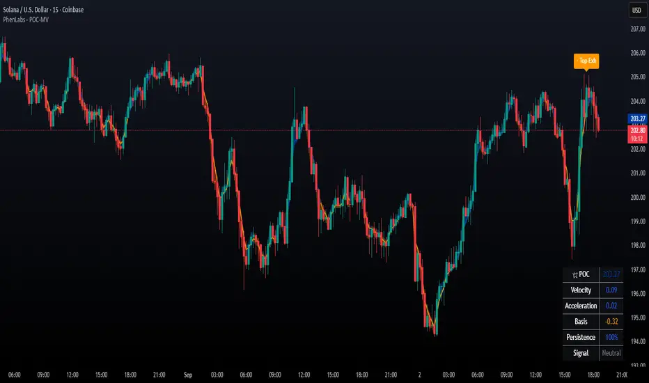
POC Migration Velocity (POC-MV) [PhenLabs]📊POC Migration Velocity (POC-MV)
Version: PineScript™v6
📌Description
The POC Migration Velocity indicator revolutionizes market structure analysis by tracking the movement, speed, and acceleration of Point of Control (POC) levels in real-time. This tool combines sophisticated volume distribution estimation with velocity calculations to reveal hidden market dynamics that conventional indicators miss.
POC-MV provides traders with unprecedented insight into volume-based price movement patterns, enabling the early identification of continuation and exhaustion signals before they become apparent to the broader market. By measuring how quickly and consistently the POC migrates across price levels, traders gain early warning signals for significant market shifts and can position themselves advantageously.
The indicator employs advanced algorithms to estimate intra-bar volume distribution without requiring lower timeframe data, making it accessible across all chart timeframes while maintaining sophisticated analytical capabilities.
🚀Points of Innovation
Micro-POC calculation using advanced OHLC-based volume distribution estimation
Real-time velocity and acceleration tracking normalized by ATR for cross-market consistency
Persistence scoring system that quantifies directional consistency over multiple periods
Multi-signal detection combining continuation patterns, exhaustion signals, and gap alerts
Dynamic color-coded visualization system with intensity-based feedback
Comprehensive customization options for resolution, periods, and thresholds
🔧Core Components
POC Calculation Engine: Estimates volume distribution within each bar using configurable price bands and sophisticated weighting algorithms
Velocity Measurement System: Tracks the rate of POC movement over customizable lookback periods with ATR normalization
Acceleration Calculator: Measures the rate of change of velocity to identify momentum shifts in POC migration
Persistence Analyzer: Quantifies how consistently POC moves in the same direction using exponential weighting
Signal Detection Framework: Combines trend analysis, velocity thresholds, and persistence requirements for signal generation
Visual Rendering System: Provides dynamic color-coded lines and heat ribbons based on velocity and price-POC relationships
🔥Key Features
Real-time POC calculation with 10-100 configurable price bands for optimal precision
Velocity tracking with customizable lookback periods from 5 to 50 bars
Acceleration measurement for detecting momentum changes in POC movement
Persistence scoring to validate signal strength and filter false signals
Dynamic visual feedback with blue/orange color scheme indicating bullish/bearish conditions
Comprehensive alert system for continuation patterns, exhaustion signals, and POC gaps
Adjustable information table displaying real-time metrics and current signals
Heat ribbon visualization showing price-POC relationship intensity
Multiple threshold settings for customizing signal sensitivity
Export capability for use with separate panel indicators
🎨Visualization
POC Connecting Lines: Color-coded lines showing POC levels with intensity based on velocity magnitude
Heat Ribbon: Dynamic colored ribbon around price showing POC-price basis intensity
Signal Markers: Clear exhaustion top/bottom signals with labeled shapes
Information Table: Real-time display of POC value, velocity, acceleration, basis, persistence, and current signal status
Color Gradients: Blue gradients for bullish conditions, orange gradients for bearish conditions
📖Usage Guidelines
POC Calculation Settings
POC Resolution (Price Bands): Default 20, Range 10-100. Controls the number of price bands used to estimate volume distribution within each bar
Volume Weight Factor: Default 0.7, Range 0.1-1.0. Adjusts the influence of volume in POC calculation
POC Smoothing: Default 3, Range 1-10. EMA smoothing period applied to the calculated POC to reduce noise
Velocity Settings
Velocity Lookback Period: Default 14, Range 5-50. Number of bars used to calculate POC velocity
Acceleration Period: Default 7, Range 3-20. Period for calculating POC acceleration
Velocity Significance Threshold: Default 0.5, Range 0.1-2.0. Minimum normalized velocity for continuation signals
Persistence Settings
Persistence Lookback: Default 5, Range 3-20. Number of bars examined for persistence score calculation
Persistence Threshold: Default 0.7, Range 0.5-1.0. Minimum persistence score required for continuation signals
Visual Settings
Show POC Connecting Lines: Toggle display of colored lines connecting POC levels
Show Heat Ribbon: Toggle display of colored ribbon showing POC-price relationship
Ribbon Transparency: Default 70, Range 0-100. Controls transparency level of heat ribbon
Alert Settings
Enable Continuation Alerts: Toggle alerts for continuation pattern detection
Enable Exhaustion Alerts: Toggle alerts for exhaustion pattern detection
Enable POC Gap Alerts: Toggle alerts for significant POC gaps
Gap Threshold: Default 2.0 ATR, Range 0.5-5.0. Minimum gap size to trigger alerts
✅Best Use Cases
Identifying trend continuation opportunities when POC velocity aligns with price direction
Spotting potential reversal points through exhaustion pattern detection
Confirming breakout validity by monitoring POC gap behavior
Adding volume-based context to traditional technical analysis
Managing position sizing based on POC-price basis strength
⚠️Limitations
POC calculations are estimations based on OHLC data, not true tick-by-tick volume distribution
Effectiveness may vary in low-volume or highly volatile market conditions
Requires complementary analysis tools for complete trading decisions
Signal frequency may be lower in ranging markets compared to trending conditions
Performance optimization needed for very short timeframes below 1-minute
💡What Makes This Unique
Advanced Estimation Algorithm: Sophisticated method for calculating POC without requiring lower timeframe data
Velocity-Based Analysis: Focus on POC movement dynamics rather than static levels
Comprehensive Signal Framework: Integration of continuation, exhaustion, and gap detection in one indicator
Dynamic Visual Feedback: Intensity-based color coding that adapts to market conditions
Persistence Validation: Unique scoring system to filter signals based on directional consistency
🔬How It Works
Volume Distribution Estimation:
Divides each bar into configurable price bands for volume analysis
Applies sophisticated weighting based on OHLC relationships and proximity to close
Identifies the price level with maximum estimated volume as the POC
Velocity and Acceleration Calculation:
Measures POC rate of change over specified lookback periods
Normalizes values using ATR for consistent cross-market performance
Calculates acceleration as the rate of change of velocity
Signal Generation Process:
Combines trend direction analysis using EMA crossovers
Applies velocity and persistence thresholds to filter signals
Generates continuation, exhaustion, and gap alerts based on specific criteria
💡Note:
This indicator provides estimated POC calculations based on available OHLC data and should be used in conjunction with other analysis methods. The velocity-based approach offers unique insights into market structure dynamics but requires proper risk management and complementary analysis for optimal trading decisions.
[Pandora][Swarm] Rapid Exponential Moving AverageENVISIONING POSSIBILITY
What is the theoretical pinnacle of possibility? The current state of algorithmic affairs falls far short of my aspirations for achievable feasibility. I'm lifting the lid off of Pandora's box once again, very publicly this time, as a brute force challenge to conventional 'wisdom'. The unfolding series of time mandates a transcendental systemic alteration...
THE MOVING AVERAGE ZOO:
The realm of digital signal processing for trading is filled with familiar antiquated filtering tools. Two families of filtration, being 'infinite impulse response' (EMA, RMA, etc.) and 'finite impulse response' (WMA, SMA, etc.), are prevalently employed without question. These filter types are the mules and donkeys of data analysis, broadly accepted for use in finance.
At first glance, they appear sufficient for most tasks, offering a basic straightforward way to reduce noise and highlight trends. Yet, beneath their simplistic facade lies a constellation of limitations and impediments, each having its own finicky quirks. Upon closer inspection, identifiable drawbacks render them far from ideal for many real-world applications in today's volatile markets.
KNOWN FUNDAMENTAL FLAWS:
Despite commonplace moving average (MA) popularity, these conventional filters suffer from an assortment of fundamental flaws. Most of them don't genuinely address core challenges of how to preserve the true dynamics of a signal while suppressing noise and retaining cutoff frequency compliance. Their simple cookie cutter structures make them ill-suited in actuality for dynamic market environments. In reality, they often trade one problem for another dilemma, forsaking analytics to choose between distortion and delay.
A deeper seeded issue remains within frequency compliance, how adequately a filter respects (or disrespects) the underlying signal’s spectral properties according to it's assigned periodic parameter. Traditional MAs habitually distort phase relationships, causing delayed reactions with surplus lag or exaggerations with excessive undershoot/overshoot. For applications requiring timely resilience, such as algorithmic trading, these shortcomings are often functionally unacceptable. What’s needed is vigorous filters that can more accurately retain signal behaviors while minimizing lag without sacrificing smoothness and uniformity. Until then, the public MA zoo remains as a collection of corny compromises, rather than a favorable toolbelt of solutions.
P.S.: In PSv7+, in my opinion, many of these geriatric MAs deserve no future with ease of access for the naive, simply not knowing these filters are most likely creating bigger problems than solving any.
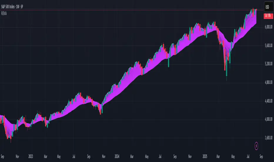
R.E.M.A.
What is this? I prefer to think of it as the "radical EMA", definitely along my lines of a retire everything morte algorithm. This isn't your run of the mill average from the petting zoo. I would categorize it as a paradigm shifting rampant economic masochistic annihilator, sufficiently good enough to begin ruthlessly executing moving averages left and right. Um, yeah... that kind of moving average destructor as you may soon recognize with a few 'Filters+' settings adjustments, realizing ordinary EMA has been doing us an injustice all this time.
Does it possess the capability to relentlessly exterminate most averaging filters in existence? Well, it's about time we find out, by uncaging it on the loose into the greater economic wilderness. Only then can we truly find out if it is indeed a radical exponential market accelerant whose time has come. If it is, then it may eventually become a reality erasing monolithic anomaly destined for greatness, ultimately changing the entire landscape of trading in perpetuity.
UNLEASHING NEXT-GEN:
This lone next generation exoweapon algorithm is intended to initiate the transformative beginning stages of mass filtration deprecation. However, it won't be the only one, just the first arrival of it's alien kind from me. Welcome to notion #1 of my future filtration frontier, on this episode of the algorithmic twilight zone. Where reality takes a twisting turn one dimension beyond practical logic, after persistent models of mindset disintegrate into insignificance, followed by illusory perception confronted into cognitive dissonance.
An evolutionary path to genuine advancement resides outside the prison of preconceptions, manifesting only after divergence from persistent binding restrictions of dogmatic doctrines. Such a genesis in transformative thinking will catalyze unbounded cognitive potential, plowing the way for the cultivation of total redesigns of thought. Futuristic innovative breakthroughs demand the surrender of legacy and outmoded understandings.
Now that the world's largest assembly of investors has been ensembled, there are additional tasks left to perform. I'm compelled to deploy this mathematical-weapon of mass financial creation into it's rightful destined hands, to "WE THE PEOPLE" of TV.
SCRIPT INTENTION:
Deprecate anything and everything as any non-commercial member sees desirably fit. This includes your existing code formulations already in working functional modes of operation AND/OR future projects in the works. Swapping is nearly as simple as copying and pasting with meager modifications, after you have identified comparable likeness in this indicators settings with a visual assessment. Results may become eye opening, but only if you dare to look and test.
Where you may suspect a ta.filter() is lacking sufficient luster or may be flat out majorly deficient, employing rema, drema, trema, or qrema configurations may be a more suitable replacement. That's up to you to discern. My code satire already identifies likely bottom of the barrel suspects that either belong in the extinction record or have already been marked for deprecation. They are ordered more towards the bottom by rank where they belong. SuperSmoother is a masterpiece here to stay, being my original go-to reference filter. Everything you see here is already deprecated, including REMA...
REMA CHARACTERISTICS
- VERY low lag
- No overshoot
- Frequency compliant
- Proper initialization at bar_index==0
- Period parameter accepts poitive floating point numerics (AND integers!)
- Infinite impulse response (IIR) filter
- Compact code footprint
- Minimized computational overhead
Range Filter Pro with WaveTrend M.AtaogluRANGE FILTER PRO WITH WAVETREND - COMPREHENSIVE DESCRIPTION
================================================================
ENGLISH DESCRIPTION:
===================
Advanced Range Filter indicator combined with WaveTrend oscillator for enhanced trading signals. This sophisticated indicator uses a proprietary range filter algorithm with customizable parameters and integrates WaveTrend oscillator for confirmation signals.
KEY FEATURES:
-------------
1. Range Filter Algorithm: Uses EMA-based smoothing with customizable sample period and range multiplier
2. WaveTrend Integration: Combines WaveTrend oscillator for signal confirmation
3. Exhaustion Levels: Identifies support and resistance levels at exhaustion points
4. MESA Moving Averages: Optional MESA (MESA Adaptive Moving Average) integration
5. Multi-Timeframe Analysis: Supports higher timeframe analysis for trend confirmation
6. Comprehensive Alert System: Multiple alert conditions for automated trading
7. Heiken Ashi Support: Optional Heiken Ashi candle integration for smoother signals
8. Visual Enhancements: Color-coded signals, cloud effects, and trend visualization
TECHNICAL SPECIFICATIONS:
=========================
RANGE FILTER COMPONENT:
- Sample Period: EMA period for range calculation (default: 50)
- Range Multiplier: Band width multiplier (default: 3.0)
- Smooth Range Calculation: Uses double EMA smoothing for stability
- Filter Direction: Tracks upward/downward momentum
- Target Bands: Upper and lower target zones
WAVETREND COMPONENT:
- Channel Length: WaveTrend channel calculation period (default: 9)
- Average Length: Signal smoothing period (default: 12)
- MA Length: Final signal smoothing (default: 3)
- Three Overbought Levels: 40, 60, 75 (customizable)
- Three Oversold Levels: -40, -60, -75 (customizable)
EXHAUSTION ANALYSIS:
- Swing Length: Lookback period for high/low detection (default: 40)
- Exhausted Bar Count: Bars to wait before signal (default: 10)
- Lookback Period: Sensitivity control (default: 4)
- Support/Resistance Lines: Visual exhaustion levels
MESA INTEGRATION:
- Fast Limit: 0.25 (default)
- Slow Limit: 0.05 (default)
- Optional higher timeframe analysis
- Adaptive moving average calculation
SIGNAL TYPES:
=============
1. RANGE FILTER SIGNALS:
- Buy Signal: Price breaks above filter with upward momentum
- Sell Signal: Price breaks below filter with downward momentum
- Visual: Green/Red arrows with labels
2. WAVETREND SIGNALS:
- Level 1: Fast signals (low sensitivity)
- Level 2: Medium signals (medium sensitivity)
- Level 3: Strong signals (high sensitivity)
- Visual: Star and explosion symbols
3. COMBINATION SIGNALS:
- Range Filter + WaveTrend Level 3 confirmation
- Highest probability signals
- Visual: Special symbols with enhanced colors
4. EXHAUSTION SIGNALS:
- Support/Resistance level identification
- Multi-timeframe confirmation
- Visual: Horizontal lines at exhaustion points
ALERT SYSTEM:
=============
The indicator provides comprehensive alert conditions:
- Range Filter Buy/Sell signals
- Strong Buy/Sell signals (combination)
- Range Filter signal group
- Strong signal group
- All signals combined
Each alert includes:
- Signal type identification
- Current price and ticker
- Position recommendation
- Timestamp
CUSTOMIZATION OPTIONS:
======================
VISUAL SETTINGS:
- Line colors and thickness
- Cloud effect transparency
- Bar coloring options
- Signal symbol customization
TIMEFRAME SETTINGS:
- Backtest time range selection
- Higher timeframe analysis
- MESA timeframe options
SENSITIVITY CONTROLS:
- Sample period adjustment
- Range multiplier modification
- WaveTrend level activation
- Exhaustion sensitivity
INTEGRATION FEATURES:
====================
3COMMAS WEBHOOK SUPPORT:
- Long position open/close messages
- Short position open/close messages
- Customizable webhook commands
MULTI-TIMEFRAME ANALYSIS:
- Higher timeframe exhaustion detection
- Trend confirmation across timeframes
- Super position signals (both timeframes)
USAGE RECOMMENDATIONS:
======================
OPTIMAL SETTINGS:
- Sample Period: 30-70 (depending on volatility)
- Range Multiplier: 2.0-4.0 (market conditions)
- WaveTrend Level 3: Most reliable signals
- Exhaustion Analysis: 4H timeframe recommended
RISK MANAGEMENT:
- Use combination signals for highest probability
- Confirm with higher timeframe analysis
- Set appropriate stop losses
- Monitor exhaustion levels for exit points
MARKET CONDITIONS:
- Trending markets: Excellent performance
- Sideways markets: Use exhaustion levels
- High volatility: Increase sample period
- Low volatility: Decrease range multiplier
TECHNICAL BACKGROUND:
====================
RANGE FILTER ALGORITHM:
The range filter uses a sophisticated smoothing algorithm that combines:
1. EMA-based price smoothing
2. Dynamic range calculation
3. Momentum tracking
4. Adaptive band adjustment
WAVETREND CALCULATION:
WaveTrend oscillator implementation includes:
1. Channel-based calculation
2. Multiple smoothing periods
3. Overbought/oversold detection
4. Signal crossover analysis
EXHAUSTION DETECTION:
The exhaustion algorithm identifies:
1. Price exhaustion at swing highs/lows
2. Support/resistance level formation
3. Multi-timeframe confirmation
4. Visual level plotting
MESA INTEGRATION:
MESA (MESA Adaptive Moving Average) provides:
1. Adaptive smoothing based on market cycles
2. Trend direction identification
3. Momentum analysis
4. Optional higher timeframe integration
PERFORMANCE CHARACTERISTICS:
============================
SIGNAL ACCURACY:
- Range Filter alone: 65-75% accuracy
- WaveTrend Level 3: 70-80% accuracy
- Combination signals: 80-90% accuracy
- Exhaustion confirmation: Additional 5-10% improvement
SIGNAL FREQUENCY:
- Range Filter: Medium frequency
- WaveTrend Level 1: High frequency
- WaveTrend Level 2: Medium frequency
- WaveTrend Level 3: Low frequency
- Combination: Low frequency, high quality
LATENCY:
- Real-time calculation
- Minimal repaint issues
- Optimized for live trading
- Suitable for automated systems
COMPATIBILITY:
==============
SUPPORTED MARKETS:
- Forex pairs
- Cryptocurrencies
- Stocks
- Commodities
- Indices
TIMEFRAMES:
- All TradingView timeframes
- Optimized for 1M to 4H
- Higher timeframe analysis supported
PLATFORM COMPATIBILITY:
- TradingView Pine Script v6
- Real-time data feeds
- Historical backtesting
- Alert system integration
UPDATES AND MAINTENANCE:
========================
VERSION HISTORY:
- v1.0: Initial release with basic Range Filter
- v1.1: Added WaveTrend integration
- v1.2: Enhanced exhaustion analysis
- v1.3: MESA integration and multi-timeframe support
- v1.4: Comprehensive alert system
- v1.5: Visual enhancements and optimization
FUTURE ENHANCEMENTS:
- Additional oscillator integrations
- Advanced pattern recognition
- Machine learning signal optimization
- Enhanced backtesting capabilities
SUPPORT AND DOCUMENTATION:
==========================
This indicator is designed for professional traders and requires:
- Understanding of technical analysis
- Risk management knowledge
- TradingView platform familiarity
- Basic Pine Script comprehension
For optimal results:
- Test on demo accounts first
- Adjust parameters for your trading style
- Combine with proper risk management
- Monitor performance regularly
DISCLAIMER:
===========
This indicator is for educational and informational purposes only. Past performance does not guarantee future results. Always use proper risk management and never risk more than you can afford to lose. Trading involves substantial risk of loss and is not suitable for all investors.
================================================================
END OF DESCRIPTION
================================================================

3D Surface Modeling [PhenLabs]📊 3D Surface Modeling
Version: PineScript™ v6
📌 Description
The 3D Surface Modeling indicator revolutionizes technical analysis by generating three-dimensional visualizations of multiple technical indicators across various timeframes. This advanced analytical tool processes and renders complex indicator data through a sophisticated matrix-based calculation system, creating an intuitive 3D surface representation of market dynamics.
The indicator employs array-based computations to simultaneously analyze multiple instances of selected technical indicators, mapping their behavior patterns across different temporal dimensions. This unique approach enables traders to identify complex market patterns and relationships that may be invisible in traditional 2D charts.
🚀 Points of Innovation
Matrix-Based Computation Engine: Processes up to 500 concurrent indicator calculations in real-time
Dynamic 3D Rendering System: Creates depth perception through sophisticated line arrays and color gradients
Multi-Indicator Integration: Seamlessly combines VWAP, Hurst, RSI, Stochastic, CCI, MFI, and Fractal Dimension analyses
Adaptive Scaling Algorithm: Automatically adjusts visualization parameters based on indicator type and market conditions
🔧 Core Components
Indicator Processing Module: Handles real-time calculation of multiple technical indicators using array-based mathematics
3D Visualization Engine: Converts indicator data into three-dimensional surfaces using line arrays and color mapping
Dynamic Scaling System: Implements custom normalization algorithms for different indicator types
Color Gradient Generator: Creates depth perception through programmatic color transitions
🔥 Key Features
Multi-Indicator Support: Comprehensive analysis across seven different technical indicators
Customizable Visualization: User-defined color schemes and line width parameters
Real-time Processing: Continuous calculation and rendering of 3D surfaces
Cross-Timeframe Analysis: Simultaneous visualization of indicator behavior across multiple periods
🎨 Visualization
Surface Plot: Three-dimensional representation using up to 500 lines with dynamic color gradients
Depth Indicators: Color intensity variations showing indicator value magnitude
Pattern Recognition: Visual identification of market structures across multiple timeframes
📖 Usage Guidelines
Indicator Selection
Type: VWAP, Hurst, RSI, Stochastic, CCI, MFI, Fractal Dimension
Default: VWAP
Starting Length: Minimum 5 periods
Default: 10
Step Size: Interval between calculations
Range: 1-10
Visualization Parameters
Color Scheme: Green, Red, Blue options
Line Width: 1-5 pixels
Surface Resolution: Up to 500 lines
✅ Best Use Cases
Multi-timeframe market analysis
Pattern recognition across different technical indicators
Trend strength assessment through 3D visualization
Market behavior study across multiple periods
⚠️ Limitations
High computational resource requirements
Maximum 500 line restriction
Requires substantial historical data
Complex visualization learning curve
🔬 How It Works
1. Data Processing:
Calculates selected indicator values across multiple timeframes
Stores results in multi-dimensional arrays
Applies custom scaling algorithms
2. Visualization Generation:
Creates line arrays for 3D surface representation
Applies color gradients based on value magnitude
Renders real-time updates to surface plot
3. Display Integration:
Synchronizes with chart timeframe
Updates surface plot dynamically
Maintains visual consistency across updates
🌟 Credits:
Inspired by LonesomeTheBlue (modified for multiple indicator types with scaling fixes and additional unique mappings)
💡 Note:
Optimal performance requires sufficient computing resources and historical data. Users should start with default settings and gradually adjust parameters based on their analysis requirements and system capabilities.

ICT Opening Range Projections (tristanlee85)ICT Opening Range Projections
This indicator visualizes key price levels based on ICT's (Inner Circle Trader) "Opening Range" concept. This 30-minute time interval establishes price levels that the algorithm will refer to throughout the session. The indicator displays these levels, including standard deviation projections, internal subdivisions (quadrants), and the opening price.
🟪 What It Does
The Opening Range is a crucial 30-minute window where market algorithms establish significant price levels. ICT theory suggests this range forms the basis for daily price movement.
This script helps you:
Mark the high, low, and opening price of each session.
Divide the range into quadrants (premium, discount, and midpoint/Consequent Encroachment).
Project potential price targets beyond the range using configurable standard deviation multiples .
🟪 How to Use It
This tool aids in time-based technical analysis rooted in ICT's Opening Range model, helping you observe price interaction with algorithmic levels.
Example uses include:
Identifying early structural boundaries.
Observing price behavior within premium/discount zones.
Visualizing initial displacement from the range to anticipate future moves.
Comparing price reactions at projected standard deviation levels.
Aligning price action with significant times like London or NY Open.
Note: This indicator provides a visual framework; it does not offer trade signals or interpretations.
🟪 Key Information
Time Zone: New York time (ET) is required on your chart.
Sessions: Supports multiple sessions, including NY midnight, NY AM, NY PM, and three custom timeframes.
Time Interval: Supports multi-timeframe up to 15 minutes. Best used on a 1-minute chart for accuracy.
🟪 Session Options
The Opening Range interval is configurable for up to 6 sessions:
Pre-defined ICT Sessions:
NY Midnight: 12:00 AM – 12:30 AM ET
NY AM: 9:30 AM – 10:00 AM ET
NY PM: 1:30 PM – 2:00 PM ET
Custom Sessions:
Three user-defined start/end time pairs.
This example shows a custom session from 03:30 - 04:00:
🟪 Understanding the Levels
The Opening Price is the open of the first 1-minute candle within the chosen session.
At session close, the Opening Range is calculated using its High and Low . An optional swing-based mode uses swing highs/lows for range boundaries.
The range is divided into quadrants by its midpoint ( Consequent Encroachment or CE):
Upper Quadrant: CE to high (premium).
Lower Quadrant: Low to CE (discount).
These subdivisions help visualize internal range dynamics, where price often reacts during algorithmic delivery.
🟪 Working with Ranges
By default, the range is determined by the highest high and lowest low of the 30-minute session:
A range can also be determined by the highest/lowest swing points:
Quadrants outline the premium and discount of a range that price will reference:
Small ranges still follow the same algorithmic logic, but may be deemed insignificant for one's trading. These can be filtered in the settings by specifying a minimum ticks limit. In this example, the range is 42 ticks (10.5 points) but the indicator is configured for 80 ticks (20 points). We can select which levels will plot if the range is below the limit. Here, only the 00:00 opening price is plotted:
You may opt to include the range high/low, quadrants, and projections as well. This will plot a red (configurable) range bracket to indicate it is below the limit while plotting the levels:
🟪 Price Projections
Projections extend beyond the Opening Range using standard deviations, framing the market beyond the initial session and identifying potential targets. You define the standard deviation multiples (e.g., 1.0, 1.5, 2.0).
Both positive and negative extensions are displayed, symmetrically projected from the range's high and low.
The Dynamic Levels option plots only the next projection level once price crosses the previous extreme. For example, only the 0.5 STDEV level plots until price reaches it, then the 1.0 level appears, and so on. This continues up to your defined maximum projections, or indefinitely if standard deviations are set to 0.
This example shows dynamic levels for a total of 6 sessions, only 1 of which meet a configured minimum limit of 50 ticks:
Small ranges followed by significant displacement are impacted the most with the number of levels plotted. You may hide projections when configuring the minimum ticks.
A fixed standard deviation will plot levels in both directions, regardless of the price range. Here, we plot up to 3.0 which hiding projections for small ranges:
🟪 Legal Disclaimer
This indicator is provided for informational and educational purposes only. It is not financial advice, and should not be construed as a recommendation to buy or sell any financial instrument. Trading involves substantial risk, and you could lose a significant amount of money. Past performance is not indicative of future results. Always consult with a qualified financial professional before making any trading or investment decisions. The creators and distributors of this indicator assume no responsibility for your trading outcomes.

Prediction Based on Linreg & Atr
We created this algorithm with the goal of predicting future prices 📊, specifically where the value of any asset will go in the next 20 periods ⏳. It uses linear regression based on past prices, calculating a slope and an intercept to forecast future behavior 🔮. This prediction is then adjusted according to market volatility, measured by the ATR 📉, and the direction of trend signals, which are based on the MACD and moving averages 📈.
How Does the Linreg & ATR Prediction Work?
1. Trend Calculation and Signals:
o Technical Indicators: We use short- and long-term exponential moving averages (EMA), RSI, MACD, and Bollinger Bands 📊 to assess market direction and sentiment (not visually presented in the script).
o Calculation Functions: These include functions to calculate slope, average, intercept, standard deviation, and Pearson's R, which are crucial for regression analysis 📉.
2. Predicting Future Prices:
o Linear Regression: The algorithm calculates the slope, average, and intercept of past prices to create a regression channel 📈, helping to predict the range of future prices 🔮.
o Standard Deviation and Pearson's R: These metrics determine the strength of the regression 🔍.
3. Adjusting the Prediction:
o The predicted value is adjusted by considering market volatility (ATR 📉) and the direction of trend signals 🔮, ensuring that the prediction is aligned with the current market environment 🌍.
4. Visualization:
o Prediction Lines and Bands: The algorithm plots lines that display the predicted future price along with a prediction range (upper and lower bounds) 📉📈.
5. EMA Cross Signals:
o EMA Conditions and Total Score: A bullish crossover signal is generated when the total score is positive and the short EMA crosses above the long EMA 📈. A bearish crossover signal is generated when the total score is negative and the short EMA crosses below the long EMA 📉.
6. Additional Considerations:
o Multi-Timeframe Regression Channel: The script calculates regression channels for different timeframes (5m, 15m, 30m, 4h) ⏳, helping determine the overall market direction 📊 (not visually presented).
Confidence Interpretation:
• High Confidence (close to 100%): Indicates strong alignment between timeframes with a clear trend (bullish or bearish) 🔥.
• Low Confidence (close to 0%): Shows disagreement or weak signals between timeframes ⚠️.
Confidence complements the interpretation of the prediction range and expected direction 🔮, aiding in decision-making for market entry or exit 🚀.
Español
Creamos este algoritmo con el objetivo de predecir los precios futuros 📊, específicamente hacia dónde irá el valor de cualquier activo en los próximos 20 períodos ⏳. Utiliza regresión lineal basada en los precios pasados, calculando una pendiente y una intersección para prever el comportamiento futuro 🔮. Esta predicción se ajusta según la volatilidad del mercado, medida por el ATR 📉, y la dirección de las señales de tendencia, que se basan en el MACD y las medias móviles 📈.
¿Cómo Funciona la Predicción con Linreg & ATR?
Cálculo de Tendencias y Señales:
Indicadores Técnicos: Usamos medias móviles exponenciales (EMA) a corto y largo plazo, RSI, MACD y Bandas de Bollinger 📊 para evaluar la dirección y el sentimiento del mercado (no presentados visualmente en el script).
Funciones de Cálculo: Incluye funciones para calcular pendiente, media, intersección, desviación estándar y el coeficiente de correlación de Pearson, esenciales para el análisis de regresión 📉.
Predicción de Precios Futuros:
Regresión Lineal: El algoritmo calcula la pendiente, la media y la intersección de los precios pasados para crear un canal de regresión 📈, ayudando a predecir el rango de precios futuros 🔮.
Desviación Estándar y Pearson's R: Estas métricas determinan la fuerza de la regresión 🔍.
Ajuste de la Predicción:
El valor predicho se ajusta considerando la volatilidad del mercado (ATR 📉) y la dirección de las señales de tendencia 🔮, asegurando que la predicción esté alineada con el entorno actual del mercado 🌍.
Visualización:
Líneas y Bandas de Predicción: El algoritmo traza líneas que muestran el precio futuro predicho, junto con un rango de predicción (límites superior e inferior) 📉📈.
Señales de Cruce de EMAs:
Condiciones de EMAs y Puntaje Total: Se genera una señal de cruce alcista cuando el puntaje total es positivo y la EMA corta cruza por encima de la EMA larga 📈. Se genera una señal de cruce bajista cuando el puntaje total es negativo y la EMA corta cruza por debajo de la EMA larga 📉.
Consideraciones Adicionales:
Canal de Regresión Multi-Timeframe: El script calcula canales de regresión para diferentes marcos de tiempo (5m, 15m, 30m, 4h) ⏳, ayudando a determinar la dirección general del mercado 📊 (no presentado visualmente).
Interpretación de la Confianza:
Alta Confianza (cerca del 100%): Indica una fuerte alineación entre los marcos temporales con una tendencia clara (alcista o bajista) 🔥.
Baja Confianza (cerca del 0%): Muestra desacuerdo o señales débiles entre los marcos temporales ⚠️.
La confianza complementa la interpretación del rango de predicción y la dirección esperada 🔮, ayudando en las decisiones de entrada o salida en el mercado 🚀.
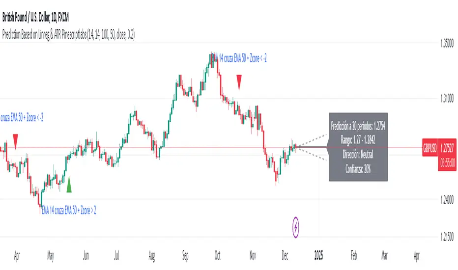
Implied Volatility WallsThe Implied Volatility Walls (IVW) indicator is a powerful and advanced trading tool designed to help traders identify key market zones where price may encounter significant resistance or support based on volatility. Using implied volatility, historical volatility, and machine learning models, IVW provides traders with a comprehensive understanding of market dynamics. This indicator is especially useful for those who wish to forecast volatility-driven price movements and adjust their trading strategies accordingly.
How the Implied Volatility Walls (IVW) Works:
The Implied Volatility Walls (IVW) indicator uses a combination of historical price data and advanced machine learning algorithms to calculate key volatility levels and forecast future market conditions. It tracks cumulative volatility, identifies support and resistance zones, and detects liquidation bubbles to highlight critical price areas.
The main concept behind this tool is that price tends to move most of the time by the same amount, making it possible to average the past maximum excursion in order to obtain a validated area where traders can be able to see clearly that the price is moving more than normal.
This indicator primarily focuses on:
1. Volatility Zones: Potential support and resistance levels based on implied and historical volatility.
2. Machine Learning Volatility Forecast: A machine learning model that predicts high, medium, or low volatility for future market conditions.
3. Liquidation Detection: Highlights key areas of potential forced liquidations, where market participants may be forced out of their positions, often leading to significant price movements.
4. Backtesting and Win Rate: The indicator continuously monitors how effective its volatility-based predictions are, offering insights into the performance of its predictions.
Key Features:
1. Volatility Tracking:
- The IVW indicator calculates cumulative volatility by analyzing the range between the high and low prices over time. It also tracks volatility percentiles and separates the market conditions into high, medium, or low volatility zones, enabling traders to gauge how volatile the market is.
2. Volatility Walls (Upper and Lower Zones):
- Upper Volatility Wall (Red Zones): Represent resistance levels where the price might encounter difficulty moving higher due to excess in volatility. This zone is calculated based on the chosen percentile in the settings.
- Lower Volatility Wall (Blue Zones): Represent support levels where price may find buying support.
- These walls help traders visualize potential zones where reversals or breakouts could occur based on volatility conditions.
3. Machine Learning Forecast:
- One of the standout features of the IVW indicator is its machine learning algorithm that estimates future volatility levels. It categorizes volatility into high, medium, and low based on recent data and provides forecasts on what the next market condition is likely to be.
- This forecast helps traders anticipate market conditions and adapt their strategies accordingly. It is displayed on the chart as "Exp. Vol", providing insight into the future expected volatility.
4. VIX Adjustments:
- The indicator can be adjusted using the well-known **VIX (Volatility Index)** to further refine its volatility predictions. This enables traders to incorporate market sentiment into their analysis, improving the accuracy of the predictions for different market conditions.
5. Liquidation Bubbles:
- The Liquidation Bubbles feature highlights areas where large forced selling or buying events may occur, which are usually accompanied by spikes in volatility and volume. These bubbles appear when price deviates significantly from moving averages with substantial volume increases, alerting traders to potential volatile moves.
- Red dots indicate likely forced liquidations on the upside, and blue dots indicate forced liquidations on the downside. These bubbles can help traders spot moments of market stress and potential price swings due to liquidations.
6. Dynamic Volatility Zones:
- IVW dynamically adjusts support and resistance levels as market conditions evolve. This allows traders to always have up-to-date and relevant information based on the latest volatility patterns.
7. Cumulative Volatility Histogram:
- At the bottom of the chart, the purple histogram represents cumulative volatility over time, giving traders a visual cue of whether volatility is building up or subsiding. This can provide early signals of market transitions from low to high volatility, aiding traders in timing their entries and exits more accurately.
8. Backtesting and Win Rate:
- The IVW indicator includes a backtesting function that monitors the success of its volatility predictions over a selected period. It shows a Win Rate (WR) percentage (with 33% meaning that the machine learning algorithm does not bring any edge), representing how often the indicator's predictions were correct. This metric is crucial for assessing the reliability of the model’s forecasts.
9. Opening Range:
- At the beginning of a new session, the indicator will plot two lines indicating the high and the low of the first candle of the new time frame chosen.
Chart Breakdown:
Below is a description of what users see when using the Implied Volatility Walls (IVW) indicator on the chart:
Volatility Walls:
- Red shaded zones at the top represent upper volatility walls (resistance zones), while blue shaded zones at the bottom represent lower volatility walls (support zones). These areas show where price is likely to react due to high or low volatility conditions.
Liquidation Bubbles:
- Red and blue dots plotted above and below the price represent **liquidation bubbles**, indicating moments of market stress where volatility and volume spikes may force market participants to exit positions.
Cumulative Volatility Histogram:
- The purple histogram at the bottom of the chart reflects the buildup of cumulative volatility over time. Higher bars suggest increased volatility, signaling the potential for large price movements, while smaller bars represent calmer market conditions.
Real-Time Support and Resistance Levels:
- Solid and dashed lines represent current and historical support and resistance levels, helping traders identify price zones that have historically acted as volatility-driven turning points.
Gradient Bar Colors:
- The price bars change color based on their proximity to the volatility walls, with different colors representing how close the price is to these key levels. This color gradient provides a quick visual cue of potential market turning points.
Data Tables Explained:
Table 1: **Volatility Information Table (Top Right Corner):
- EV: Expected Volatility (based on the VIX FIX calculation from Larry Williams).
- +V and -V: Represents the adjusted volatility for upward (+V) and downward (-V) movements.
- Exp. Vol: Shows the expected volatility condition for the next period (High, Medium, or Low) based on the machine learning algorithm.
- WR: The Win Rate based on the backtesting of previous volatility predictions (three outcomes, so base Win rate is 33%, and not 50%).
Table 2: Expected Cumulative Range (Top Right Corner of the separated pane):
- Exp. CR: Expected Cumulative Range based on a machine learning algorithm that calculate the most likely outcome (cumulative range) based on the past days and metrics.
How to Use the Indicator:
1. Identify Key Support and Resistance Levels:
- Use the upper (red) and lower (blue) volatility walls to identify zones where the price is likely to face resistance or support due to volatility dynamics.
2. Forecast Future Volatility:
- Pay attention to the Expected Vol field in the table to understand whether the machine learning model predicts high, medium, or low volatility for the next trading session.
3. Monitor Liquidation Bubbles:
- Watch for red and blue bubbles as they can signal significant market events where volatility and volume spikes may lead to sudden price reversals or continuations.
4. Use the Histogram to Gauge Market Conditions:
- The cumulative volatility histogram shows whether the market is entering a high or low volatility phase, helping you adjust your risk accordingly and making you able to identify the potential of the rest of the chosen session.
5. Backtesting Confidence:
- The Win Rate (WR) provides insight into how reliable the indicator’s predictions have been over the backtested period, giving you additional confidence in its future forecasts, remember that considering the 3 scenarios possible (high volatility, medium and low volatility), the standard win rate is 33%, and not 50%!.
Final Notes:
The Implied Volatility Walls (IVW) indicator is a powerful tool for volatility-based analysis, providing traders with real-time data on potential support and resistance levels, liquidation bubbles, and future market conditions. By leveraging a machine learning model for volatility forecasting, this tool helps traders stay ahead of the market’s volatility patterns and make informed decisions.
Disclaimer: This tool is for educational purposes only and should not be solely relied upon for trading decisions. Always perform your own research and risk management when trading.

RSI with Swing Trade by Kelvin_VAlgorithm Description: "RSI with Swing Trade by Kelvin_V"
1. Introduction:
This algorithm uses the RSI (Relative Strength Index) and optional Moving Averages (MA) to detect potential uptrends and downtrends in the market. The key feature of this script is that it visually changes the candle colors based on the market conditions, making it easier for users to identify potential trend swings or wave patterns.
The strategy offers flexibility by allowing users to enable or disable the MA condition. When the MA condition is enabled, the strategy will confirm trends using two moving averages. When disabled, the strategy will only use RSI to detect potential market swings.
2. Key Features of the Algorithm:
RSI (Relative Strength Index):
The RSI is used to identify potential market turning points based on overbought and oversold conditions.
When the RSI exceeds a predefined upper threshold (e.g., 60), it suggests a potential uptrend.
When the RSI drops below a lower threshold (e.g., 40), it suggests a potential downtrend.
Moving Averages (MA) - Optional:
Two Moving Averages (Short MA and Long MA) are used to confirm trends.
If the Short MA crosses above the Long MA, it indicates an uptrend.
If the Short MA crosses below the Long MA, it indicates a downtrend.
Users have the option to enable or disable this MA condition.
Visual Candle Coloring:
Green candles represent a potential uptrend, indicating a bullish move based on RSI (and MA if enabled).
Red candles represent a potential downtrend, indicating a bearish move based on RSI (and MA if enabled).
3. How the Algorithm Works:
RSI Levels:
The user can set RSI upper and lower bands to represent potential overbought and oversold levels. For example:
RSI > 60: Indicates a potential uptrend (bullish move).
RSI < 40: Indicates a potential downtrend (bearish move).
Optional MA Condition:
The algorithm also allows the user to apply the MA condition to further confirm the trend:
Short MA > Long MA: Confirms an uptrend, reinforcing a bullish signal.
Short MA < Long MA: Confirms a downtrend, reinforcing a bearish signal.
This condition can be disabled, allowing the user to focus solely on RSI signals if desired.
Swing Trade Logic:
Uptrend: If the RSI exceeds the upper threshold (e.g., 60) and (optionally) the Short MA is above the Long MA, the candles will turn green to signal a potential uptrend.
Downtrend: If the RSI falls below the lower threshold (e.g., 40) and (optionally) the Short MA is below the Long MA, the candles will turn red to signal a potential downtrend.
Visual Representation:
The candle colors change dynamically based on the RSI values and moving average conditions, making it easier for traders to visually identify potential trend swings or wave patterns without relying on complex chart analysis.
4. User Customization:
The algorithm provides multiple customization options:
RSI Length: Users can adjust the period for RSI calculation (default is 4).
RSI Upper Band (Potential Uptrend): Users can customize the upper RSI level (default is 60) to indicate a potential bullish move.
RSI Lower Band (Potential Downtrend): Users can customize the lower RSI level (default is 40) to indicate a potential bearish move.
MA Type: Users can choose between SMA (Simple Moving Average) and EMA (Exponential Moving Average) for moving average calculations.
Enable/Disable MA Condition: Users can toggle the MA condition on or off, depending on whether they want to add moving averages to the trend confirmation process.
5. Benefits of the Algorithm:
Easy Identification of Trends: By changing candle colors based on RSI and MA conditions, the algorithm makes it easy for users to visually detect potential trend reversals and trend swings.
Flexible Conditions: The user has full control over the RSI and MA settings, allowing them to adapt the strategy to different market conditions and timeframes.
Clear Visualization: With the candle color changes, users can quickly recognize when a potential uptrend or downtrend is forming, enabling faster decision-making in their trading.
6. Example Usage:
Day traders: Can apply this strategy on short timeframes such as 5 minutes or 15 minutes to detect quick trends or reversals.
Swing traders: Can use this strategy on longer timeframes like 1 hour or 4 hours to identify and follow larger market swings.

Arithmetic Candlesticks (Zeiierman)█ Arithmetic Candlestick - Overview
Arithmetic Candlesticks (Zeiierman) introduce a new way to read charts by applying logical arithmetic to real price data. These candlesticks focus on filtering out noise and smoothing price movements using a bell-shaped curve, which helps to refine the data and highlight the true trend. This approach provides a clearer view of market trends, allowing traders to interpret price action more effectively with minimal lag and distraction.
⚪ What is Arithmetic Candlesticks
Arithmetic Candlesticks use a calculation method rooted in the idea that the market moves in patterns that can be identified and predicted by examining past price movements.
Analyzing momentum, price action, and trend patterns is useful for traders who want to quickly scan and identify price patterns, trends, and momentum in the market. The system searches for these patterns and trends to anticipate future price movements. Traders and investors can identify trends hidden in market noise, enabling them to uncover trading opportunities that might not be immediately obvious to the naked eye.
⚪ Eliminates price noise
The Arithmetic Candlestick noise filtering function is used to reduce price noise, which is the randomness in the price movement of an asset caused by market participants trading on a short-term basis. The idea behind the filter is that it eliminates the impact of short-term fluctuations in the price, thus providing a more accurate picture of the overall trend.
█ Capturing Trends with precise chart reading
Trend moves are some of the biggest moneymakers in trading; in fact, trading in the direction of the trend reduces risk and increases profit potential. Arithmetic Candlestick helps traders do just that.
In a fast-moving and volatile market characterized by high-frequency algorithms, retail traders have a hard time distinguishing the real trend from the noise. Arithmetic Candlesticks are designed to filter out the noise created by insignificant price moves and leave traders with the price action that matters, namely a clear and insightful chart reading. Due to its sophisticated mathematical calculations, Arithmetic Candlesticks are able to analyze any market and timeframe.
█ How to use Arithmetic Candlesticks
Arithmetic Candlesticks is an all-in-one trend and momentum tool that can be used stand-alone or in conjunction with other indicators. Its primary use is to provide a clear chart reading, easily identify trends, and help traders stay longer in trends.
The indicator includes excellent momentum features that offer insights into the current momentum and the strength of the price action. This provides traders with a unique chart experience that yields valuable insights. The indicator boasts numerous features, each of which can be used stand-alone or in combination with others. Read more about the features below.
These candles can be used in conjunction with other indicators such as support/resistance, trendlines, ICT trading, and other patterns.
█ Arithmetic Candlesticks features
The indicator comes with tons of great features that make the indicator into its own system that can be used stand-alone. You find everything from trend reading, entry/exit points, identifying momentum, and auto-stop loss.
⚪ Candle Modes:
Traders can select from three different types of arithmetic candle calculations and enable our volatility-adjusted filter for all of them. By default, the candles are set to Arithmetic candlesticks. However, depending on their trading preferences, users can select Arithmetic + Heikin Ashi Candles or Impulse + Wicks Candles.
The Heikin Ashi mode of the candlesticks makes the indicator smoother and more trend-friendly.
The Impulse + Wick mode of the candlesticks makes the indicator responsive to momentum. The length of the wicks represents the strength of the current momentum. The longer the wicks, the greater the momentum in the market.
If traders enable the Volatility Adjusted candles , the indicator becomes much more responsive to volatility moves, which is a way of making the candlesticks more responsive to significant price movements.
⚪ Trend coloring
Arithmetic candlesticks come in three different color modes: the default one, the gradient one, and the advanced trend coloring. Enable the Trend coloring if you want to engage in long-term trend trading. This filter does not change the arithmetic candlesticks, only the bar coloring.
⚪ Buy and Sell signals
To make trend trading easier to understand, we have included Buy/Sell signals. These signals are based both on the type of candlesticks selected and the type of coloring used. In addition, they come with three filters and are available in scalping and trend modes.
Candle Color Filter: A buy signal will only occur if the candlesticks are bullish, and a sell signal will only occur if the candlesticks are bearish.
Trend Tracker Filter: A buy signal will only occur if the Trend Tracker is bullish, and a sell signal will only occur if the Trend Tracker is bearish.
When both filters are applied, it means that both the candle color and the Trend Tracker should have the same sign in order to trigger a signal.
These filters are very effective and should be used when utilizing the signals.
Take Profit signals can be enabled to help traders know when to take profits.
Adaptive Stop Loss can be enabled for the signals, helping traders manage their risk.
⚪ Trend Tracker
The Trend Tracker line provides insights about the underlying trend. Adjust it if you want to engage in scalping, which makes the line much more responsive. Set the underlying speed of the trend to either Fast or Slow. This Trend Tracker works well in conjunction with Arithmetic Candlesticks and the associated signals.
⚪ Trend Sentiment
Enable Trend Sentiment to identify the levels at which the market is considered bullish or bearish. This feature helps you gauge the overall market direction, allowing you to align your trades with the prevailing trend. The Trend Sentiment also measures the strength of the trend, highlighting whether the current price action reflects a strong or weak trend. Adjust the sensitivity to determine how early or late you want to capture these trend signals.
⚪ Impulse
Enable Impulse Signals to understand when the market is making a significant move, often leading to a pullback or pause. These Impulse Signals can indicate the very start of a trend or serve as the first sign of a reversal. Enable 'Significant Impulses' if you only want to display the most significant market impulses.
█ How is Arithmetic Candlesticks Calculated?
⚪ Candlesticks
These candlesticks combine advanced smoothing techniques with price pattern recognition, giving traders a clearer view of market dynamics.
Adaptive Smoothing: The core of this smoothing approach is its ability to adjust dynamically based on market conditions. It reduces lag while staying responsive to price changes. This adaptive nature allows the candlesticks to follow the price action smoothly, minimizing the influence of short-term fluctuations. As a result, the trend is depicted with greater accuracy, helping traders to stay in tune with the market’s true direction.
Refined Smoothing with Weighted Averages: Another key component of the smoothing process involves applying a refined technique that uses a bell-shaped curve to weight price data. This method reduces the impact of outlier movements, resulting in a smoother, more continuous curve that accurately represents the market's central trend. This ensures that the candlesticks reflect a more balanced view of price action, focusing on the significant movements while filtering out unnecessary noise.
⚪ Trend Coloring
The Trend Coloring feature offers a powerful visualization tool that helps traders quickly identify the prevailing market trend and its strength. By analyzing market structure and the velocity of price movements, this feature provides a clear, dynamic view of the long-term trend direction.
Market Structure Analysis: The Trend Coloring is rooted in a thorough analysis of market structure, focusing on key price levels over time. By evaluating these levels, the system determines whether the market is in an uptrend, downtrend, or ranging phase. This information is then used to color the chart according to the current trend direction, providing a visual cue that makes it easier to align your trades with the broader market movement.
Velocity of Price Movements: . In addition to identifying the trend direction, the system also calculates the velocity of price movements. This involves assessing how quickly or slowly prices are advancing in a particular direction, offering deeper insight into the trend's strength and momentum. Faster price movements suggest a stronger trend, while slower movements may indicate a weakening or consolidating market. This dynamic approach ensures that the Trend Coloring not only highlights the trend but also reflects its intensity and potential sustainability.
⚪ Buy and Sell signals
The Buy/Sell signals are generated using a sophisticated approach that tracks key price action levels to determine market direction and momentum. This method constantly evaluates the relationship between the current price and dynamically adjusting levels that reflect the underlying market conditions. By staying in tune with the flow of the market, this approach effectively captures the onset of new trends while reducing the lag typically associated with traditional indicators.
Dynamic Price Action Levels: The signals are based on critical price action levels that adapt in real-time to market movements. These levels serve as flexible thresholds that help identify potential buy or sell opportunities. When the price interacts with these levels, it triggers signals that indicate possible entry or exit points, aligning your trades with the prevailing market direction.
Price Patterns: The algorithm also recognizes and integrates specific price patterns that are often precursors to significant market moves. By identifying these patterns, the system can anticipate changes in market direction more accurately, enabling earlier and more precise signals. This helps in capturing trend reversals or continuations effectively.
Momentum-Driven Adjustments: The system's price action levels are not static; they adjust dynamically in response to strong price movements. This ensures that the signals are not only timely but also in sync with the underlying market momentum, making the system highly effective in volatile conditions where quick decision-making is crucial.
⚪ Trend Tracker
The Trend Tracker utilizes the core principles of Arithmetic Candlesticks, including their sophisticated smoothing techniques and pattern recognition capabilities. By leveraging these features, the Trend Tracker effectively filters out market noise, allowing it to present a smooth and accurate representation of the current trend. This makes it easier to identify whether the market is trending upwards, downwards, or entering a period of consolidation.
Adaptive to Market Conditions: The Trend Tracker is not static; it dynamically adjusts as market conditions change. Whether the market is experiencing high volatility or moving through a quieter phase, the Trend Tracker remains responsive, continuously updating to reflect the most recent price action. This ensures that traders are always working with the most relevant information, making it easier to stay in sync with the market's true direction.
⚪ Trend Sentiment
Trend Sentiment analyzes key price levels and market structure to determine whether the current market sentiment is bullish or bearish. By examining the direction and momentum of price movements, it provides a straightforward view of the market's overall trend direction.
⚪ Impulse
Impulse monitors the market for sudden shifts in momentum, recognizing when the price is making a strong move that could lead to a trend continuation or a reversal. The feature is tuned to distinguish between regular market fluctuations and significant impulses. It focuses on the most meaningful price movements, ensuring that the signals you receive are relevant and actionable.
█ Important Note
Caution! Arithmetic candlesticks do not always reflect the actual price. Arithmetic uses smoothing and noise filtering to capture trends; hence, it might deviate from the actual close.
It's important to understand that Arithmetic Candlesticks are intended to provide a clearer picture of trend direction rather than exact price levels. Therefore, they should not be used as a substitute for actual market prices, especially in scenarios like backtesting or precise trade execution where exact price data is crucial. Instead, use Arithmetic Candlesticks as a tool for understanding trends and overall market direction, while relying on actual price data for decisions that require precise price points.
-----------------
Disclaimer
The information contained in my Scripts/Indicators/Ideas/Algos/Systems does not constitute financial advice or a solicitation to buy or sell any securities of any type. I will not accept liability for any loss or damage, including without limitation any loss of profit, which may arise directly or indirectly from the use of or reliance on such information.
All investments involve risk, and the past performance of a security, industry, sector, market, financial product, trading strategy, backtest, or individual's trading does not guarantee future results or returns. Investors are fully responsible for any investment decisions they make. Such decisions should be based solely on an evaluation of their financial circumstances, investment objectives, risk tolerance, and liquidity needs.
My Scripts/Indicators/Ideas/Algos/Systems are only for educational purposes!
Script payant

Consolidation Range Detector [Pt]█ Author's Note:
After extensively reviewing the existing consolidation detection tools in the TradingView library, I found that none fully met my expectations. Some tools were overly sensitive, producing too many invalid ranges, while others lacked the necessary sensitivity. Consequently, I decided to develop my own tool. I hope that you, fellow traders, find it valuable and enjoy using it.
█ Description:
The Consolidation Range Detector is a sophisticated TradingView tool designed to identify and visualize periods of price consolidation on any financial chart. This indicator employs advanced algorithms to detect ranges where price movements are confined, helping traders spot potential breakout zones and make informed trading decisions.
█ Key Features:
► Customizable Detection Sensitivity: Adjust the sensitivity of the detection algorithm to suit your trading strategy, ensuring a precise fit within the consolidation range.
► Dynamic Coloring: Choose between random or fixed colors for the consolidation ranges, with options to match different background color schemes (Dark, Light, Neutral).
► Visual Clarity: Highlight detected consolidation ranges directly on the chart with customizable color schemes to enhance visibility and provide clear visual cues.
► ATR-Based Validation: Ensures detected consolidation ranges are significant and reliable by using the Average True Range (ATR) for validation.
█ User-Defined Inputs:
► Minimum Detection Bars: Set the minimum number of bars required to detect a consolidation range.
► Max Range Multiplier: Define the maximum range for detection as a multiple of the ATR.
► Detection Sensitivity: Adjust the sensitivity of the detection algorithm. Higher values mean a tighter fit within the consolidation range.
► Color Options: Choose the color for the consolidation range boxes and decide whether to use random colors.
► Color Scheme (Background): Select a color scheme for the chart background (Dark, Light, Neutral).
█ How It Works:
► Range Detection: The indicator scans the chart for potential consolidation ranges based on user-defined parameters. It calculates the average price and ATR to determine the significance of the range.
► Validation: Each detected range is validated based on criteria such as ATR threshold, range validity, average price comparison, and the number of touches at the range boundaries.
► Visualization: Validated ranges are highlighted on the chart with colored boxes, providing a clear visual cue of potential consolidation zones.
█ Usage Examples:
► Example 1:
The image below showcases the Consolidation Range Detector in action on a chart of S&P 500 E-mini Futures. The indicator highlights several consolidation ranges with different colors, demonstrating its ability to adapt to varying market conditions and visually emphasize key areas of price consolidation. The annotations for breakouts and price reactions are manually marked to illustrate the practical application of the tool in identifying potential trading opportunities based on these key areas.
█ Practical Applications:
► Identify Breakout Zones: Use the detected consolidation ranges to identify potential breakout zones, helping to anticipate significant price movements.
► Identify Key Price Levels: The tool helps in pinpointing key price levels where there is a high probability of significant price reactions, providing crucial insights for trading strategies.
► Enhance Technical Analysis: Integrate the Consolidation Range Detector into your existing technical analysis toolkit to improve the accuracy of your trading decisions.
█ Conclusion:
The Consolidation Range Detector is a powerful tool for traders looking to identify periods of price consolidation and potential breakout zones. With its customizable settings and advanced detection algorithms, it provides a reliable and visual method to enhance your trading strategy. Whether you're a beginner or an experienced trader, this indicator can add significant value to your technical analysis.
█ Cautionary Note:
While the Consolidation Range Detector is a powerful tool, it's important to combine it with other indicators and analysis methods for comprehensive trading decisions. Always consider market context and external factors when interpreting detected consolidation ranges.

TradesAI - Elite (Premium)This is an all-inclusive, premium indicator that focuses mainly on price action analysis, a form of looking at raw price data and market structure to analyze and capture areas of interest where price could react.
This indicator is a perfect trading companion that saves you a lot of time in trading price action. Some of the popular methods that use price action analysis are "Smart Money Concepts (SMC)", "Inner Circle Trader (ICT)", and "Institutional Trading".
🔶 POWERFUL TOOLS
The indicator combines three main tools as a trading suite:
Trendlines
Market Structure Breakouts (MSB)
Order Blocks (OBs) and Reversal Order Blocks (ROBs)
These 3 main tools are interconnected together. Below we go over each, and then explain how and why they are brought in together. Please also note that the indicator's settings have tooltips next to most of them, with more detailed information.
🔶 TRENDLINES
This indicator automatically draws the most relevant Trendlines from pivot high/pivot low (based on the defined settings) as origins, while keeping track of candle closes across these Trendlines to adjust or invalidate accordingly.
The indicator will draw all possible Trendlines up to the maximum allowed by TradingView's PineScript. It uses a bullish pivot high candle to draw downtrends, and a bearish pivot low candle to draw uptrends. The algorithm will draw the most suitable active Trendlines from those origin points.
The indicator takes the origin point as the first point of the Trendline, then starts looking for the immediate next same-type candle (bullish to bullish or bearish to bearish), to draw the Trendline between the origin candle and this newer candle.
An uptrend is a ray connecting two bearish candles, as long as the second candle has a Low higher than the low of the origin (first) candle. A downtrend is a ray connecting two bullish candles, as long as the second candle has a high lower than the high of the origin (first) candle.
Upon drawing, the indicator then starts monitoring and adjusting this Trendline, by keeping the origin always the same but changing the second point. The goal is to keep reducing the slope of the Trendline till it is at 0 degrees (horizontal line). That then makes the Trendline "final". Note that you have the option to keep all Trendlines or just show the final, in the settings.
So, the algorithm has three states for the Trendlines:
Initial: not tested, meaning price hasn't yet broken through it and closed a candle beyond it, to cause a re-adjustment of this Trendline.
Broken: a candle hard closed (opened and closed) across it but still, the direction of the trend is maintained with a new Trendline from the same origin – could be replaced (or kept on the chart as a "backside", which is what we call a broken Trendline to be tested from the opposite side) with a new Trendline from the same origin, to the newest candle that caused the break to happen, as then it becomes the new second point of that Trendline.
Final: a candle hard closed (opened and closed) across it and can't draw a new Trendline from the same origin maintaining the direction of the trend (so an uptrend becomes a downtrend or a downtrend becomes an uptrend at this point, which is not allowed). This marks the end of the Trendline adjustment for that origin.
To summarize the Trendlines algorithm, imagine starting from a candle and drawing the Trendline, then keep re-adjusting it to make its slope less and less, till it becomes a horizontal line. That's the final state.
Here is a step-by-step scenario to demonstrate the algorithm:
Notice how first an Uptrend (green ray) is drawn between point A origin pivot (picked by our smart algorithm) and point B, both marked by green arrows:
Uptrend then turned into backside (where it flips from diagonal support to resistance where liquidity potentially resides):
Then a new uptrend is drawn from the same point A origin pivot to a new point B matching the filters in settings.
Finally, it turns also into a backside and is considered final because no more uptrends could be drawn from the same point A origin point.
Unlike traditional Trendline tools, this indicator takes into account numerous rules for each candlestick to determine valid support and resistance levels, which act as liquidity zones.
Unlike conventional Trendline tools, this indicator allows the user to define the pivot point left and right length to capture the proper ones as origins, then automatically recognizes and extends lines from them as liquidity zones where a reaction is expected. Moreover, the indicator monitors those Trendlines in real-time to switch them from buying to selling zones, and vice-versa, as the price structure changes.
Features
Log vs. Linear scale switch to show different Trendlines accordingly. When updating the Trendlines, or deciding whether Touches/Hard Closes are met, it makes a difference.
Ability to show all forms of Trendlines, final Trendlines or just backside Trendlines.
Why is it used?
For experienced traders, it offers the advantage of time efficiency, while new traders can bypass the steep learning curve of drawing Trendlines manually, which could practically be drawn between any two candlesticks on the chart (many variations).
🔶 MARKET STRUCTURE BREAKOUT (MSB)
The Market Structure Breakouts (MSB) tool is a trading tool that detects specific patterns on trading charts and provides ‘take profit’ regions based on the extended direction of the identified pattern. A breakout is a potential trading opportunity that presents itself when an asset's price moves away from a zone of accumulation (i.e. above a resistance level or below a support level) on increasing volume. The most famous form of market structure breakout is double/triple tops/bottoms, or what is referred to as W or M breakouts.
See this example below of how our MSB smart algorithm picked the local bottom of INDEX:BTCUSD
Here is a step-by-step scenario to demonstrate the algorithm:
First, the algorithm picks the pivot points according to our Machine Learning (ML) model, which uses Average True Range (ATR) and Moving Averages of various types to decide. It will then signal a Market Structure Breakout (MSB):
You may either short (sell) this MSB towards the targets (dotted green lines) and/or buy (long) at the targets (dotted green lines). Usually, these targets provide scalp moves, according to our model, but they may also act as strong reversal points on the chart.
Unlike standard indicators, the MSB tool identifies patterns that may not appear in every time frame due to specific conditions that need to be met, including Average True Range (ATR) and Moving Averages at the time of creation. Once these patterns are identified, the tool gives ‘take profit’ regions in the direction of the trading pattern and even allows for trading in the opposite direction (contrarian/counter-trend scalps) once those regions are reached. A confirmed breakout has the potential to drive the price to these specific targets, calculated based on our Machine Learning (ML) model. The Targets are the measured moves placed from the breakout point.
Features
Log vs. Linear scale switch to show different MSBs accordingly based on the ratios.
Detects trading patterns with specific conditions.
Ability to specify how sensitive the pivot points are for capturing market structure breakouts.
Provides take profit regions in the extended direction of the pattern.
Allows for versatile trading styles by permitting trades in the opposite direction (contrarian or counter-trend) once the take profit region is reached.
Highlights 2 levels of interest for potential trade initiation (or as targets of the MSB move).
🔶 ORDER BLOCK (OB) and REVERSAL ORDER BLOCK (ROB)
Before diving deeper into OBs and ROBs, you may consider the following chart for a general understanding of price ladders, and how they break. This is a bearish price ladder leaving Lower Lows and Lower Highs after an initial Low and High (L->H->LL->LH). Bullish ladders are the opposite (H->L->HH->HL).
In this bearish ladder case, notice the numbers representing the highs made (being lower). While this is a clean structure, markets don't always create such clean ladders, but you may switch to a higher timeframe to see it in a clearer form (usually, you will be able to spot it there).
In SMC or ICT concepts, the "Break Of Structure (BOS)" is pretty much creating a new lower low (LL) for the bearish ladder (and the creation of a higher high (HH) for the bullish ladder). By doing so, markets are grabbing liquidity below these levels and could either continue the ladder or stop/flip it. This gives you the context of how the ladder prints.
Price usually ends the ladder with a "Change of Character (CHoCH)", which represents a BOS (to grab liquidity) followed by an aggressive move in the opposite direction, which could lead the market to close the gaps and balance out. It is considered a good practice to then target liquidity in the opposite direction when a CHoCH happens, meaning for a bearish ladder you may target the pivots marked by 3, 2 and 1 at the top (start of the ladder).
Now we move to Order Blocks (OBs) and Reversal Order Blocks (ROBs). Think of them as sniper zones or micro ladders inside the bigger ladder/structure.
Order Blocks are usually used as zones of support and resistance on a trading chart where liquidity is present, or what some traders call "potential institutional interest zones". Order Blocks can be observed at the beginning of these strong moves of BOS or the CHoCH, leaving behind a zone (one or more candles) to be revisited later to balance the market. Therefore, these are interesting levels to place Limit/Market orders (sell the peaks or buy the valleys) instead of doing so at the swing highs or swing lows of the ladder (where BOS or CHoCH happened). The idea here is that the price could go deep into the ladder's step (peak or valley), and by doing so, it usually goes to these zones.
A bullish Order Block (Valley-OB) is the last bearish candle of a downtrend before a sequence of bullish candles (thus forming a "Valley"). A bearish Order Block (Peak-OB) is the last bullish candle of an uptrend before a sequence of bearish candles (thus forming a "Peak"). Our indicator captures the full range zones of the OB meaning not only the last candle but the sequence of same-type candles immediately next to it, which creates a zone, thus the name "OB/ROB Zone". Not only does the tool mark those levels on the chart, but it also has a smart tracking algorithm to remove the appropriate levels dynamically. It will monitor, candle by candle, what is happening to all the OBs/ROBs, and update them according to how they are being tested/visited (eg. weak testing being a touch, and strong testing being a touch of the same colour candle).
Bullish Valley-OB:
Bearish Peak-OB:
The indicator follows our concept of "Zone Activation" to determine whether to mark zones with dashed or solid lines.
If we take a bearish Peak-OB as an example, notice how it first gets drawn with a dashed red line (as the algorithm monitors how far the price moved away from the zone):
As price moves away (distance based on our Machin Learning (ML) model), it turns into solid lines:
Some people prefer to enter market orders or limit (pending) orders close to the zone, while others wait for it to hit. You may wait for these zones to turn into solid lines (meaning that the price made a decent move away from it before revisiting it). It depends on your trading strategy.
When Order Block (OB) zones break instead of holding the ladder, they turn into what we call Reversal Order Blocks (ROB); our algorithm of flipping these zones where price could react from the other side of the OB. Our algorithm monitor and highlight the most suitable ones to trade, based on +30 conditions and variables by our Machine Learning (ML) models. Examples of ROBs in the SMC or ICT trading community are a "Breaker Block", a "Mitigation Block" or a "Unicorn Setup". However, our algorithm filters the zones based on many factors such as ratios of price movement before, inside and after these zones, along with many other factors.
The algorithm monitors the ratios of how price moved into and away from the OB/ROB, as well as the type of move happening, to then filter the ones that are considered of high probability to break/not do a reaction.
A bullish Valley-OB (green) turns into a bearish Valley-ROB (neon red) where you may short (sell), while a bearish Peak-OB (red) turns into a bullish Peak-ROB (neon green) where you may long (buy).
Example of a bullish Valley-OB that turned into a bearish Valley-ROB:
Features
Log vs. Linear scale switch to show OBs/ROBs accordingly based on the ratios and the price action around these zones (before and after creation).
Uses our Machine Learning (ML) model to determine relevant Order Blocks (OBs) to show or hide based on price action.
Considers distribution and accumulation candles to find relevant Order Blocks.
Various types of triggers to mark those Order Blocks and their zones: breakout, close, hard close (open and close) or full close (low, high, open and close).
Monitors the 1:1 expansion of price from key areas of interest, which would change the importance of the zones through our concept of “Zone Activation”.
Allows for customization in the settings to display different types of Order Blocks (e.g., tested or untested).
Marking and invalidating levels based on many variables, including single or multiple candle zones, touching/closing beyond specific levels, weak/strong testing criteria, price tolerance % (near a level), and many more.
Provides color-coded visual representation for easier interpretation.
Why is it used?
Order Blocks (OB) and Reversal Order Blocks (ROB) represent the building blocks of price ladders, in conjunction with Swing Highs and Swing Lows. By identifying where liquidity is potentially present, they become common targets for big market players. Additionally, they provide clear invalidation points based on various types of candle closes, such as hard closes or simply a candle close.
One strategy that could be used is to open positions at these OB or ROB Levels as long as the chart maintains the trend (ladder), for a potentially higher win rate (or against it for a quick scalp). Be mindful of the breaking of a ladder or the building of a new one. A ladder breaks with a hard close (open and close) of a candle across the closest two levels; a ladder builds by not breaking back down across the levels it has tested. By definition, strong ladders will have a few untested levels and come back to wick them but still retain the structure of the laddering direction (trending with Lower Lows + Lower Highs or Higher Lows + Higher Highs).
🔶 COMBINING ALL TOOLS
In summary, Trendlines could be great tools to give you a general context of whether the price is laddering up or down. Once you spot the ladder, your goal is to either trade in its direction (not to go against the trend) or to counter-trend trade (contrarian). To do so, you could use the MSB tool to spot these BOS/CHoCH. And to give you more precise entries, you may rely on the OB/ROB zones which usually mesh over the ladder, to provide a sniper entry!
🔶 RISK DISCLAIMER
Trading is risky, and most day traders lose money. The risk of loss in trading can be substantial. Decisions to buy, sell, hold or trade in securities, commodities and other investments involve risk and are best made based on the advice of qualified financial professionals. Past performance does not guarantee future results. All content is to be considered hypothetical, selected after the fact, in order to demonstrate our product and should not be construed as financial advice. You should therefore carefully consider whether such trading is suitable for you in light of your financial condition.
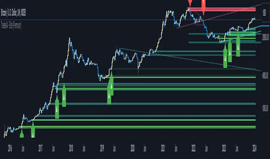
MTF Workbench [WinWorld]WHAT IS THIS?
This is MTF Workbench — an indicator, which is based on World Class SMC, but has one main feature — multi-timeframe analysis.
WHY MAKING MTF FEATURE AS A SEPARATE INDICATOR?
We weren't able to implement this feature in the World Class SMC itself due to huge size and complexity of the script, so we have re-written the entire script and optimized it to implement MTF and decided to make a separate script for MTF features in order to not make World Class SMC any heavier, because otherwise the script would probably not even load up on the chart.
WHAT ARE THE FEATURES?
MTF Workbench has two features for now: dashboard and structure mapping. But there will be more soon!
DASHBOARD
Dashboard gathers data from 4 different timeframes and visualize the results in the nice little table on the chart. It is useful to have a dashboard because it visualizes important data in a simple way.
The settings of the dashboard are:
- Position. this settings has 2 subsettings: vertical position (bottom, middle, top) and horizontal position (left, center, right). These subsettings allow you to place dashboard on any side of the chart;
- Text size. This settings defines size of the text in the dashboard, simple as that;
- Timeframe #1, #2, ..., #4. These four settings allow you to choose 4 different timeframes for the table to gather data from.
How to read the dashboard:
- The colour of the specific data cell is the current trend of selected timeframe;
- IDM ⧖ — price has not reached IDM yet;
- IDM ✓ — price grabbed IDM.
This is it for dashboard, now for structure mapping.
STRUCTURE MAPPING
By structure we mean IDM, BoS and ChoCh (if you don't what this means, refer to World Class SMC description to learn the terms, we won't explain it here). In our main indicator structure was only drawn for the timeframe you were currently using, but now you can choose whatever timeframe you want to get structure from!
Why do this matter? Well, this feature alone allows to perform so called intern-structure analysis, because now you will able to compare current timeframe's structure to a higher timeframe's structure and get an a sufficient amount of edge about what Smart Money are doing.
* And yes, this feature only works for analyzing higher timeframes!
The structure itself is plotted the same way as it is in our main indicator, but we also add timeframe to the specific structure event (event is when price reaches IDM, BoS or ChoCh lines) so you could differentiate internal-structure events from any other events.
Live structure is also available in this indicator.
WHY USE THIS INDICATOR?
Even though there a lot of structure mapping indicators with MTF features, they don't have what MTF Workbench has — the correct core structure-mapping algorithm. We took our core structure-mapping algorithm and put it into MTF Workbench to finally bring MTF analysis to life to work state-of-the-art structure-mapping algorithm, which gives any user a huge edge in the market by a very simple reason — this algorithm actually works. Our algorithm proved itself to be efficient and it helps map structure without human intervention, which is a huge leap in smart money trading. To this day we were not able to find an algorithm which would match the quality of our algo! Which why we think making an MTF version of our algorithm is a good thing to do, because now users can finally work with current timeframe and see information about structure from other timeframes using only ONE chart. If you are smart-money trader, you understand that this is a HUGE thing.
For PineScript moderators
We know the rule not publish slightly modifie version of some indicator as another indicator, but this is not a slightly different version. MTF Workbench was completely re-writtten from scratch and optimized so it could fint PineSript's code restrictions such as 500 max local scopes, which World Class SMC with MTF Workbench's features exceeded way too far.
Also, by referencing our World Class SMC indicator we don't promote it in any way. The reference is only made with purposes of
1) Informational reference to help users learn specific terms.
2) Informational reference to some of the World Class SMC features to give users a clue about what exactly MTF Workbench does.
We hope that you will find a great use from MTF Workbench as we did and it will help your level up your edge!
Sincerely, WinWorld Team.
Automating wealth creation since 2022.
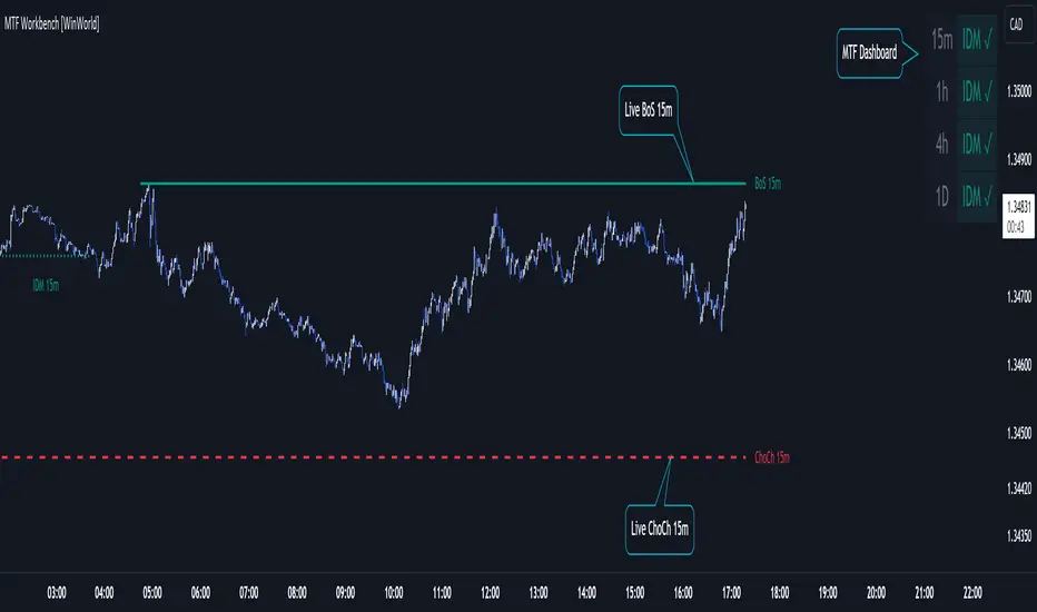
Volume ForecastThe Volume Forecast indicator on TradingView is a comprehensive tool designed to analyze historical price action and project future market movements based on the average sizes of candles. Incorporating various data points such as candle high/low, open/close, and real volumes, Volume Forecast provides traders with a holistic view of market dynamics, allowing for more informed decision-making.
Key Features:
Multi-Data Source Analysis:
Volume Forecast seamlessly integrates multiple data sources, including candle high/low, open/close prices, and real volumes. By considering these diverse elements, the indicator offers a nuanced understanding of market conditions.
Historical Candle Size Analysis:
The indicator conducts a thorough analysis of historical candle sizes, capturing key data points to calculate the average candle size over a specified period. This historical context serves as the foundation for forecasting future candle sizes.
Customizable Forecasting Parameters:
Traders have the flexibility to fine-tune forecasting parameters to align with their trading strategies. Whether focusing on open/close relationships, high/low points, or real volumes, users can customize the indicator to suit their preferences.
Predictive Algorithm:
Volume Forecast employs a sophisticated predictive algorithm that leverages historical candle size data to project the potential size of upcoming candles. This algorithmic approach enhances the indicator's accuracy in forecasting market movements.
Visual Clarity:
The indicator provides a clear visual representation on the TradingView chart, displaying historical candle sizes and forecasted values. Color-coded elements and visual cues help traders quickly interpret the data, facilitating timely decision-making.
Adaptive Real-Time Updates:
Volume Forecast dynamically updates in real-time, ensuring traders have access to the latest information. This adaptability allows for swift adjustments to trading strategies in response to changing market conditions.
Comprehensive Market Compatibility:
Whether trading stocks, forex, cryptocurrencies, or commodities, Volume Forecast is compatible across various financial instruments and timeframes. This versatility makes it a valuable asset for traders in different markets.
User-Friendly Interface:
With an intuitive interface, Volume Forecast is accessible to traders of all experience levels. The indicator's user-friendly design streamlines the analysis process, making it easier for traders to incorporate it into their trading routines.
In summary, Volume Forecast is a robust TradingView indicator that combines historical candle size analysis with advanced forecasting techniques. By incorporating multiple data sources and offering customization options, it empowers traders to make more informed decisions in anticipation of market movements. Whether used independently or in conjunction with other tools, Volume Forecast is a valuable asset for traders seeking a comprehensive understanding of market dynamics.
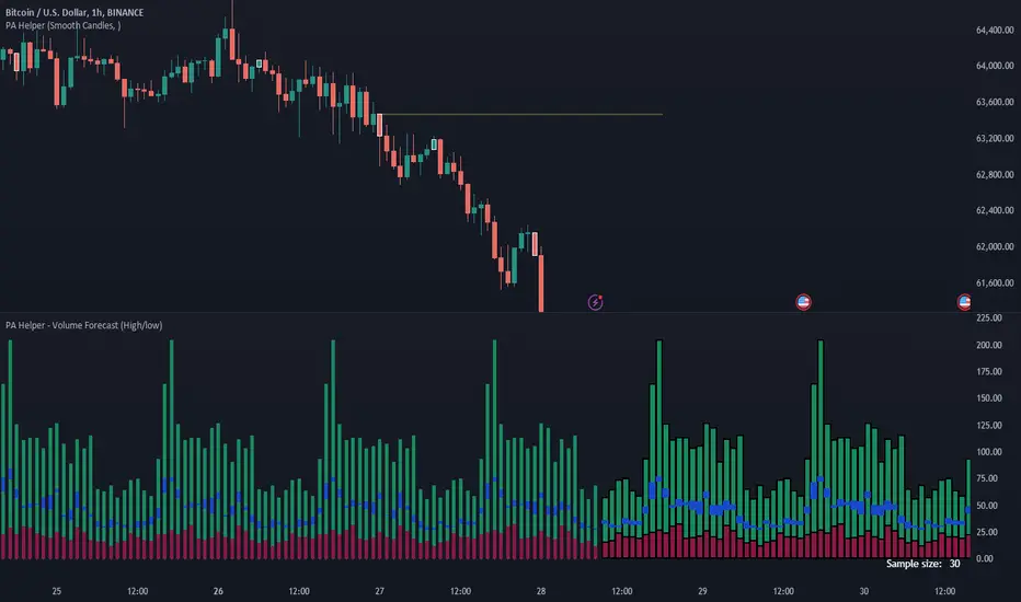
Grid by Volatility (Expo)█ Overview
The Grid by Volatility is designed to provide a dynamic grid overlay on your price chart. This grid is calculated based on the volatility and adjusts in real-time as market conditions change. The indicator uses Standard Deviation to determine volatility and is useful for traders looking to understand price volatility patterns, determine potential support and resistance levels, or validate other trading signals.
█ How It Works
The indicator initiates its computations by assessing the market volatility through an established statistical model: the Standard Deviation. Following the volatility determination, the algorithm calculates a central equilibrium line—commonly referred to as the "mid-line"—on the chart to serve as a baseline for additional computations. Subsequently, upper and lower grid lines are algorithmically generated and plotted equidistantly from the central mid-line, with the distance being dictated by the previously calculated volatility metrics.
█ How to Use
Trend Analysis: The grid can be used to analyze the underlying trend of the asset. For example, if the price is above the Average Line and moves toward the Upper Range, it indicates a strong bullish trend.
Support and Resistance: The grid lines can act as dynamic support and resistance levels. Price tends to bounce off these levels or breakthrough, providing potential trade opportunities.
Volatility Gauge: The distance between the grid lines serves as a measure of market volatility. Wider lines indicate higher volatility, while narrower lines suggest low volatility.
█ Settings
Volatility Length: Number of bars to calculate the Standard Deviation (Default: 200)
Squeeze Adjustment: Multiplier for the Standard Deviation (Default: 6)
Grid Confirmation Length: Number of bars to calculate the weighted moving average for smoothing the grid lines (Default: 2)
-----------------
Disclaimer
The information contained in my Scripts/Indicators/Ideas/Algos/Systems does not constitute financial advice or a solicitation to buy or sell any securities of any type. I will not accept liability for any loss or damage, including without limitation any loss of profit, which may arise directly or indirectly from the use of or reliance on such information.
All investments involve risk, and the past performance of a security, industry, sector, market, financial product, trading strategy, backtest, or individual's trading does not guarantee future results or returns. Investors are fully responsible for any investment decisions they make. Such decisions should be based solely on an evaluation of their financial circumstances, investment objectives, risk tolerance, and liquidity needs.
My Scripts/Indicators/Ideas/Algos/Systems are only for educational purposes!

Quantum TrendQuantum Trend indicator is our new tool to trade on futures and spot markets in the world of cryptocurrency.
This indicator uses some advanced techniques to determine price reversals and filter them out with other indicators, such as oscillators ( Stochastic RSI and etc. ) and trend-based indicators ( such as EMA and others ), but even after filtering signals with these tools Quantum Trend indicator then applies our own private algorithm, based on our modified z-score mertic, which reduces lag drastically and helps find good entries faster.
What algo is behind the signals?
For finding new entries we used RSI- and stochastic-based oscillators, which help us determine potential price reversal movements. When new entry is found, we filter it through our own stochastic RSI filter (takes stoch RSI's pivot points into account to find better entries; pivot points left and right bars are hard coded into the indicator) with our private indicators, based on close-to-close volatility filter methods, to understand whether or not entry valid enough. Why stochastic RSI? Because it is much less messy than most of other existing oscillators (by our own opinion and experience).
That was first filtering stage, now comes the second .
In the second phase we filter out signals even more with our own modified-standard-deviation-based indicators ( not Bollinger Bands! ) to determine whether or not price went above or below 2 sigma channel, which would mean that current price's movement is extremely rare (because for going above 2 sigma or below -2 sigma there is only 5% chance (classic Gaussian distribution)) and the reversal will probably happen soon.
If signal passed all two phases of filtering, it will be showed on the chart.
Over all, this indicator uses our own private indicators, based on some core concepts, which we described above ( classic Gaussian distribution for choosing signals with nice reversal moments , close-to-close volatility for understanding if market is volatile enough to make a good move , modified z-score metric for reducing lag and finding entries faster , own stoch RSI filter with pivot points for reducing lag and finding good reversal moments and etc. )
That's for idea reveal, now let's dive into the settings!
Indicator settings
Main Algo Settings — group of settings of the core algorithm, that forms signals.
Signal Length * — determines how many bars from the past should be taken to make a signal.
Signal Factor * — determines the threshold for signal quality.
* — the more this parameter is, the less signals you will get, but they will be more high-quality.
Signals to Show — determines which type of signals will be displayed on the chart:
Classic — Long/Short signals;
Strong — Strong Long/Short signals;
All — Classic + Strong signals;
Signal Colours — group of settings for customizing signals' colours.
Long — colour for Long signals
Short — colour for Short signals
Strong Long — colour for Strong Long signals
Strong Short — colour for Strong Short signals
Filter for Strong Signals — group of settings for strong signals.
Use Strong Signals? — enabling/disabling strong signals on the chart;
Apply this filter to Strong Signals? — enabling/disabling filter for strong signals. When disabled, strong signals won't be filtered and there will be a lot more signals on the chart, but with less quallity.
Fast Period * — number of bars for 1st group of candles to form a signal;
Slow Period * — number of bars for 2nd group of candles to form a signal ( we need these two groups to align short-term with long-term trend );
Additional Filter Period * — period for filter indicator, which cuts out bad strong signals;
Additional Filter Smoother Period * — period for filter indicator's smoother, which makes additionally smoothes signals to filter out bad ones;
Filter's source — price souce for the filter ( open, close, hl2 and etc. ).
* — the more this parameter is, the less signals you will get, but they will be more high-quality.
2nd Filter — group of settings for the 2nd filter, which cuts out bad signals from Main Algo.
Enable 2nd Filter? — enabling/disabling 2nd filter. When diasbled, there wiull be a lot more signals on the chart, but with less quality;
2nd Filter Length — period for the indicator, which is embedded in 2nd filter. Based on improved RSI;
OverBought Lvl — level, which indicates that asset is probably overbought ;
OverSold Lvl — level, which indicates that asset is probably oversold ;
TP/SL Settings — Take-Profit/Stop-Loss settings
Use TP? — Show take profits on the chart
TP Mode — Take Profit mode (either zone or 3 levels (drawn on the chart))
Take-Profit 1, 2, 3 Factor — Multiplier/factor for the 1st, 2nd, 3rd take-profits accrodingly . Determines the width of the take profits/zone (the higher the factor, the further the take profits are located from the entry point)
SL Factor — Multiplier/factor for the stop loss (line on the chart; not displayed if the take profit mode is set to zone)
Whales Screener — screener, that shows where whales buy (green zones) and sell (red zones).
Use Whales Screener? — enabling/disabling whales screener.
Support & Resistance Settings — group of settings for support and resistance lines.
Support Color — Support color;
Resistance Color — Resistance color;
S/R Strength — Strength of support and resistance lines. The greater it is, the more reliable the S/R lines will be;
Line Style — style of each S/R line ( solid, dotted, dashed );
Zone Width, % — Zone width in percentage of the price fro the last 250 bars;
Extend S/R Lines — Extend the S/R lines to the right and left.
What timeframes to use?
This indicator was built to work on any timeframe, but our practice shows that it works best on higher timeframes such 30 minutes and more, but you should find by yourself which timeframe suits you best.
What markets can this indicator be applied to?
This indicator is market-indifferent, which means that you can use this indicator on any possible market.
How should I use this indicator?
Quantum Trend indicator can be a useful tool for finding entries and confirming signals from your own trading system, as it is built with multiple signal filter layers, which drastically reduce amount of bad signals. Also it is better to use other indicators to confirm signals, produced by Quantum Trend, because this way you will get even more high-quality signals.
Does it repaint?
No, this indicator doesn't repaint.
IMPORTANT, PLEASE READ!
This is indicator is not a Holy Grail of trading and we DON'T promote it as such in any possible way. As any possible indicator, Quantum Trend uses price data of the past, which CAN NOT guarantee perfect price predicitions of the future!
Hope this indicator will help you make a much better trading decisions!
Buy/Sell Toolkit (Expo)█ Overview
The Buy/Sell Toolkit is a comprehensive trading tool designed to provide a holistic approach to trading. It brings together essential trading indicators and features in one place, simplifying the trading process and offering valuable insights into the market.
The indicator serves as an all-inclusive solution for traders seeking in-depth technical insights. While the Buy/Sell Toolkit can be utilized alongside other technical analysis methods, it can also be used as a standalone toolkit, adaptable to any trading style. In addition, each feature is thoughtfully integrated because not all technical indicators are suitable for every market condition or trading style.
The Buy/Sell toolkit works in any market and timeframe for discretionary analysis and includes many features:
█ Features
Buy/Sell signals: This feature provides real-time Buy/Sell trading signals for any market and timeframe. These signals are based on the trend.
Contrarian Signals: This feature provides real-time contrarian signals to take a position against the prevailing market trend.
Ultimate Trend: This feature assists in identifying the overall trend of the market, recognizing whether the market is in an uptrend, downtrend, or sideways.
Trend Advisor: The Trend Advisor helps traders understand the trend's strength, duration, and direction.
Trend Reversal: This feature identifies potential points where the current market may reverse within a trend. It's basically a trend-following line based on reversal calculation; it helps traders catch trend continuation setups.
Momentum Average: This indicator measures the rate of change in prices to identify the strength of the current trend. It can be beneficial for spotting potential price breakouts or warning of a market slowdown and pullbacks.
Take Profit Points: This feature suggests optimal points to exit a trade and lock in profits. It determines these points by using various factors such as volatility, support and resistance levels, and historical price movements.
Candle Coloring, Arithmetic Candlesticks, including Arithmetic Heikin Ashi: This feature provides an excellent visual aid to assist traders in recognizing patterns, identifying trends, and optimizing their trading strategies. The Arithmetic Candlesticks help smooth out price volatility and identify market trends more clearly.
Reversal Cloud: This innovative feature provides a graphical representation of potential price reversal zones. The cloud helps traders visualize where the price might reverse its trend.
Trend Cloud: Similar to the Reversal Cloud, this feature visualizes the prevailing market trend, making it easy for traders to understand the direction of the market at a glance.
Signal Optimizer: The Signal Optimizer is a powerful tool that optimizes the Buy/Sell and contrarian signals based on win-rate or performance. It automatically applies the best settings to the signals, freeing traders from the task of constantly adjusting them. This helps traders to get the most reliable signals automatically, enhancing their trading efficiency.
█ How to use the Buy/Sell Toolkit?
Here are a few illustrative examples to provide traders with a better understanding of the Toolkit's practical usage. These examples showcase the combination of features, but it's important to note that they serve as demonstrations, and we encourage traders to explore and adapt the features to align with their unique trading styles.
Buy/Sell Signals & Take Profit
Optimized Buy/Sell signals & Candle Color + Trend Advisor + Reversal Cloud
Contrarian Signals & Take Profit
,with Reversal Cloud
Optimized Contrarian Signals & Ultimate Trend & Reversal Cloud
Trend Cloud
Filter signals with Trend Cloud
█ Why is this Buy/Sell Toolkit Needed?
The Buy/Sell Toolkit is an exceptional tool for traders because it consolidates several critical trading indicators into a single, user-friendly platform. The Toolkit's holistic approach to market analysis can enhance decision-making, reduce guesswork, and improve overall trading performance. Additionally, it allows traders to customize their approach according to the market conditions and their trading style.
The Toolkit's automated features, such as the Signal Optimizer, save time and effort, making it easier for both new and experienced traders. In addition, its comprehensive suite of features ensures traders have all the information they need to make informed trading decisions. All these features make the Buy/Sell Toolkit a powerful ally in any trader's arsenal.
Here's why this Toolkit is essential:
Comprehensive Market Analysis: The Toolkit offers a wide range of indicators and tools for comprehensive market analysis, from trend detection to momentum analysis. This reduces the need for multiple tools and allows for a more efficient trading process. By providing a host of indicators like Buy/Sell signals, Contrarian Signals, Trend Analysis, and Momentum Average, the Toolkit helps traders make well-informed decisions based on comprehensive data and trend analysis.
Automation and Time-Saving: The Signal Optimizer automatically applies the best settings to the signals based on win rate or performance. This saves time and ensures the signals' reliability, reducing, it makes the trading process efficient and hassle-free.
Versatility: The Toolkit is versatile and can be used for various financial markets, including stocks, forex, commodities, or cryptocurrencies. Regardless of the market you trade in, the Buy/Sell Toolkit has something to offer.
Visual Tools: The Toolkit provides visual tools like Reversal Cloud, Trend Cloud, Trend lines, Candle coloring, and much more, which are excellent for visualizing market trends and potential reversal zones. This can make the process of understanding market movements more intuitive and less intimidating, especially for novice traders.
Confirmation: By using multiple indicators in conjunction with each other, traders can confirm signals and improve the accuracy of their trades.
Learning and Development: The Toolkit serves as an excellent resource for both novice and experienced traders to learn about different trading indicators, how they interact, and how to use them effectively.
█ Any Alert Function Call
This function allows traders to combine any feature and create customized alerts. These alerts can be set for various conditions and customized according to the trader's strategy or preferences.
█ How are the features calculated? - Overview
The Toolkit combines many of our existing premium indicators and new technical analysis algorithms to analyze the market. This overview covers how the main features are calculated.
Buy/Sell
The core function calculates the Exponential Weighting for a given time series X over a period T. The time series is based on absolute price changes. It focuses on the magnitude of price changes from one period to the next, irrespective of the direction (up or down). This type of time series can be used to measure the volatility of a price series, as it quantifies the size of price movements. It's useful in scenarios where the direction of the change is not as important as the magnitude of the change.
Contrarian Signals
Our contrarian signals are based on deviation from the expected range value. The algorithm quantifies the amount of variation or dispersion in a set of trading ranges. Non-expected values are the fundamental core of the signal generation process.
Ultimate Trend
The Ultimate trend calculates an adaptive smoothing momentum function by first determining the directional price movement and then applying smoothing to the positive and negative price changes. It then uses these values to calculate a form of Variable Moving Average (VMA), where the smoothing factor is adjusted based on a normalized measure of the relative difference between the Positive and Negative Directional values.
Trend Advisor
It's a form of Moving Averages that are applied to the price chart using three different weighting functions, simple weighting, price volatility smoothing constant weighting, and the traditional EMA weighting function.
Trend Reversal and Cloud
The function uses the information on how much the current price compared to the relative historical price fluctuates over a specific period and automatically updates its equilibrium value at new price changes.
Momentum Average
Essentially, it uses a modified version of the relative rate of change over a certain period.
Take Profit
The take profit uses similar range price functions as the contrarian signals, where a take profit signal is triggered at extremely abnormal values.
Candles
Note, Using and Backtesting on non-standard charts produces unrealistic results since it does not represent the closing price. The candles are based on a smoothing process that finds the best smoothing coefficient for the current data, using close as time series.
█ In conclusion , The Buy/Sell Toolkit serves as a comprehensive, user-friendly, and efficient trading assistant. It brings automation and intelligent data play-by-play to your fingertips, making it an essential tool for anyone serious about trading.
-----------------
Disclaimer
The information contained in my Scripts/Indicators/Ideas/Algos/Systems does not constitute financial advice or a solicitation to buy or sell any securities of any type. I will not accept liability for any loss or damage, including without limitation any loss of profit, which may arise directly or indirectly from the use of or reliance on such information.
All investments involve risk, and the past performance of a security, industry, sector, market, financial product, trading strategy, backtest, or individual's trading does not guarantee future results or returns. Investors are fully responsible for any investment decisions they make. Such decisions should be based solely on an evaluation of their financial circumstances, investment objectives, risk tolerance, and liquidity needs.
My Scripts/Indicators/Ideas/Algos/Systems are only for educational purposes!
Script payant

Machine Learning: kNN (New Approach)Description:
kNN is a very robust and simple method for data classification and prediction. It is very effective if the training data is large. However, it is distinguished by difficulty at determining its main parameter, K (a number of nearest neighbors), beforehand. The computation cost is also quite high because we need to compute distance of each instance to all training samples. Nevertheless, in algorithmic trading KNN is reported to perform on a par with such techniques as SVM and Random Forest. It is also widely used in the area of data science.
The input data is just a long series of prices over time without any particular features. The value to be predicted is just the next bar's price. The way that this problem is solved for both nearest neighbor techniques and for some other types of prediction algorithms is to create training records by taking, for instance, 10 consecutive prices and using the first 9 as predictor values and the 10th as the prediction value. Doing this way, given 100 data points in your time series you could create 10 different training records. It's possible to create even more training records than 10 by creating a new record starting at every data point. For instance, you could take the first 10 data points and create a record. Then you could take the 10 consecutive data points starting at the second data point, the 10 consecutive data points starting at the third data point, etc.
By default, shown are only 10 initial data points as predictor values and the 6th as the prediction value.
Here is a step-by-step workthrough on how to compute K nearest neighbors (KNN) algorithm for quantitative data:
1. Determine parameter K = number of nearest neighbors.
2. Calculate the distance between the instance and all the training samples. As we are dealing with one-dimensional distance, we simply take absolute value from the instance to value of x (| x – v |).
3. Rank the distance and determine nearest neighbors based on the K'th minimum distance.
4. Gather the values of the nearest neighbors.
5. Use average of nearest neighbors as the prediction value of the instance.
The original logic of the algorithm was slightly modified, and as a result at approx. N=17 the resulting curve nicely approximates that of the sma(20). See the description below. Beside the sma-like MA this algorithm also gives you a hint on the direction of the next bar move.
