Visible Range Volume Profile Heatmap [MyTradingCoder]The Visible Range Volume Profile Heatmap indicator offers a visually striking and insightful way to analyze trading volume within the visible price range of your chart. This tool goes beyond traditional volume profiles by displaying volume distribution as a heatmap, where color intensity represents the volume traded at each price level.
Key Features:
Dynamic Heatmap: Displays volume concentration using a color gradient, making it easy to spot areas of high and low trading activity.
Customizable Grid: Choose between auto-scaling or manual grid configuration to suit your analysis needs.
Flexible Color Schemes: Select from tri-tone or two-tone color palettes to represent bullish and bearish volume.
Point of Control (POC) Overlay: Highlights the price level with the highest trading volume, a critical reference point for traders.
Adjustable Transparency: Fine-tune the visibility of the heatmap to balance it with other chart elements.
Lookback Period: Customize the number of bars used for volume profile calculation.
How to Use the Visible Range Volume Profile Heatmap:
The Visible Range Volume Profile Heatmap is a powerful tool that can significantly enhance your market analysis when used effectively. To get the most out of this indicator, start by observing the overall pattern of the heatmap. Areas with darker colors represent higher volume concentration, indicating price levels where significant trading activity has occurred. These areas often serve as important support or resistance levels, as they represent prices where many traders have established positions.
Pay close attention to the Point of Control (POC), represented by a line running through the heatmap. This line marks the price level with the highest trading volume and often acts as a magnet for price action. Price tends to gravitate towards the POC, making it a crucial reference point for potential reversals or continuations.
When analyzing potential trades, consider how the current price relates to the volume distribution shown in the heatmap. If the price is approaching a high-volume area from below, it might face resistance; conversely, if it's approaching from above, that area might provide support. Breakouts beyond significant volume nodes can be particularly noteworthy, as they may signal a shift in market sentiment.
Use the heatmap in conjunction with your existing trading strategies. For example, if you're a trend follower, you might look for breakouts beyond major volume areas as confirmation of trend continuation. If you're a mean reversion trader, you might consider entries when price moves away from high-volume nodes, anticipating a return to these heavily traded levels.
The indicator can also help in identifying potential profit targets. As price moves away from one volume node, it often continues until it reaches the next significant volume area. These areas can serve as logical places to consider taking profits or adjusting your position.
For longer-term analysis, observe how the volume profile changes over time. Shifts in the distribution of volume can indicate evolving market dynamics. A broadening of the high-volume area might suggest increasing uncertainty, while a narrowing could indicate building consensus about price.
Settings Explained:
Auto Grid Configuration:
The "Auto Scale" option automatically adjusts the grid size based on the visible chart area. This ensures optimal visualization regardless of your chart's dimensions or zoom level.
Auto Scale Grid Size: Determines the total number of cells in the heatmap. A higher number provides more granular detail but may increase calculation time.
Auto Scale Grid Ratio: Adjusts the aspect ratio of the grid cells. A higher ratio creates wider, more rectangular cells, while a lower ratio results in more square-shaped cells. Experiment to find the best visual representation for your analysis.
Lookback Period:
The lookback setting determines how many columns (bars) of historical data the indicator uses to calculate the volume profile. A larger lookback will provide a more comprehensive view of historical volume distribution but may be slower to react to recent changes. A smaller lookback will be more responsive to recent volume patterns but may miss longer-term trends.
Manual Grid Configuration:
If you prefer more control over the grid layout, you can switch to manual configuration:
Column Width: Sets the number of price bars each column of the heatmap represents. A wider column aggregates more data, smoothing out the profile.
Number of Rows: Determines the vertical resolution of the heatmap. More rows provide finer price level detail but may make the overall pattern less distinct.
Tips for Optimization:
For short-term trading, use a smaller lookback and finer grid settings to capture recent market dynamics.
For longer-term analysis, increase the lookback and use wider columns to identify persistent volume patterns.
If the heatmap appears too blocky, increase the number of rows or decrease the column width.
If the heatmap is too granular, making patterns hard to discern, do the opposite.
Remember, the ideal settings often depend on your specific trading timeframe, the asset you're analyzing, and your personal analytical preferences. Don't hesitate to experiment with different configurations to find what works best for your trading style.
Conclusion
The Visible Range Volume Profile Heatmap is more than just an indicator—it's a versatile tool that enhances your ability to analyze and interpret market data. By transforming volume profiles into an intuitive, color-coded heatmap, this indicator allows you to quickly identify critical price levels where significant trading activity has occurred. Whether you're a day trader focused on short-term moves or a swing trader analyzing longer-term trends, the customizable settings of this tool provide the flexibility needed to adapt to various market conditions.
The ability to configure the grid layout, adjust the lookback period, and fine-tune the color and transparency settings ensures that the heatmap can be tailored to your specific trading strategy. By highlighting key areas of support and resistance, identifying potential breakouts, and pinpointing the Point of Control (POC), the heatmap gives you actionable insights that can enhance your decision-making process.
Incorporate the Visible Range Volume Profile Heatmap into your trading routine to gain a deeper understanding of market dynamics and to spot opportunities that might otherwise go unnoticed. Remember to experiment with the settings to find the configuration that best suits your analysis style, and use this powerful indicator in conjunction with your existing strategies for optimal results. With the right approach, this tool can become an indispensable part of your trading toolkit, helping you navigate the markets with greater confidence and precision.
Recherche dans les scripts pour "grid"

Market Sector Scanner/Screener With MOM + RSI + MFI + DMI + MACDMARKET SECTOR SCANNER/SCREENER MOM + RSI + MFI + DMI + MACD FOR STOCKS CRYPTO & FOREX
This script scans 9 markets constantly and returns the values of 5 different popular indicators.
This indicator helps you see when one of your favorite stocks is bullish or bearish when you are not watching that chart so you can always catch the big moves as they happen.
***HOW TO USE***
A great way to use this market screener is to set up separate chart layouts for each sector you like to trade. Such as the top 9 stocks in the S & P 500, top 9 stocks in the XLF etf, etc. Make sure to set up separate chart layouts in Tradingview so you don’t have to change the symbols constantly. This will give you a good idea in real time if that entire sector is bullish, bearish or mixed. When the entire grid goes red or green, those are very strong signs of market direction across that entire sector, so trades in the corresponding direction are quite safe.
This can be done for crypto as well, using the top 9 cryptocurrencies by market cap. Watch the grid and wait for the entire lot to turn green or red and then take a position in that direction.
You can also use this with a variety of your favorite tickers so you can see when specific markets are looking strong in either direction, instead of constantly changing charts or missing good opportunities because you weren’t watching that specific chart.
This grid can also be used to determine how long to hold a position as well. If the entire grid is still green or red, according to your trade direction, you can usually expect price to continue in that direction until you see some conflicting colors start to pop up on the grid. As it starts to give mixed signals, you can expect the market to be indecisive or reverse which is a good time to get out.
If you have your scanner setup to show similar markets in one sector, be careful taking trades when the grid is very mixed in color. This shows signs of indecision and will likely have choppy price action until the market decides a direction so make sure to use caution when the grid is mixed. It is best to wait for the entire grid to turn green or red and then take position.
***COLOR MEANINGS***
When each indicator value is in bullish territory, the background of that value will turn green.
When each indicator value is in bearish territory, the background of that value will turn red.
When each indicator value is in neutral territory, the background of that value will turn blue.
When all 5 indicators for a ticker are bullish, the ticker background will turn green.
When all 5 indicators for a ticker are bearish, the ticker background will turn red.
When there is a mixture of bullish and bearish values, the ticker background will turn blue.
***CUSTOMIZATION***
You can customize which tickers are in your scanner including stocks, crypto, futures and forex, the source of the indicators, the length of the indicator settings and the smoothing parameters.
***INDICATORS USED***
The indicators used for each ticker are as follows:
Momentum(MOM) - Default length is 14. Bullish is above zero, bearish is below zero.
Relative Strength Index(RSI) - Default length is 14. Bullish is above 50, bearish is below 50.
Money Flow Index(MFI) - Default length is 14. Bullish is above 50, bearish is below 50.
Directional Movement Index(DMI) - Default length is 14 and smoothing is 14. Calculated by subtracting di minus from di plus. If the value is positive, it is bullish. If the value is negative, it is bearish.
Moving Average Convergence & Divergence(MACD) - Default settings are 12, 26, 9. If the short line is greater than the long line, then it is bullish. If the short line is less than the long line, it is bearish.
***MARKETS***
This market scanner can be used as a signal on all markets, including stocks, crypto, futures and forex.
***TIMEFRAMES***
This scanner can be used on all timeframes and pulls data from other tickers using the same timeframe as what your current chart is set to.
***TIPS***
Try using numerous indicators of ours on your chart so you can instantly see the bullish or bearish trend of multiple indicators in real time without having to analyze the data. Some of our favorites are Trend Friend Scalp & Swing Signals, Auto Fibonacci, Directional Movement Index, Volume Profile With Buy/Sell Pressure, Auto Support And Resistance and Money Flow Index in combination with this Scanner. They all have real time Bullish and Bearish labels as well so you can immediately understand each indicator's trend.

Quantum Rotational Field MappingQuantum Rotational Field Mapping (QRFM):
Phase Coherence Detection Through Complex-Plane Oscillator Analysis
Quantum Rotational Field Mapping applies complex-plane mathematics and phase-space analysis to oscillator ensembles, identifying high-probability trend ignition points by measuring when multiple independent oscillators achieve phase coherence. Unlike traditional multi-oscillator approaches that simply stack indicators or use boolean AND/OR logic, this system converts each oscillator into a rotating phasor (vector) in the complex plane and calculates the Coherence Index (CI) —a mathematical measure of how tightly aligned the ensemble has become—then generates signals only when alignment, phase direction, and pairwise entanglement all converge.
The indicator combines three mathematical frameworks: phasor representation using analytic signal theory to extract phase and amplitude from each oscillator, coherence measurement using vector summation in the complex plane to quantify group alignment, and entanglement analysis that calculates pairwise phase agreement across all oscillator combinations. This creates a multi-dimensional confirmation system that distinguishes between random oscillator noise and genuine regime transitions.
What Makes This Original
Complex-Plane Phasor Framework
This indicator implements classical signal processing mathematics adapted for market oscillators. Each oscillator—whether RSI, MACD, Stochastic, CCI, Williams %R, MFI, ROC, or TSI—is first normalized to a common scale, then converted into a complex-plane representation using an in-phase (I) and quadrature (Q) component. The in-phase component is the oscillator value itself, while the quadrature component is calculated as the first difference (derivative proxy), creating a velocity-aware representation.
From these components, the system extracts:
Phase (φ) : Calculated as φ = atan2(Q, I), representing the oscillator's position in its cycle (mapped to -180° to +180°)
Amplitude (A) : Calculated as A = √(I² + Q²), representing the oscillator's strength or conviction
This mathematical approach is fundamentally different from simply reading oscillator values. A phasor captures both where an oscillator is in its cycle (phase angle) and how strongly it's expressing that position (amplitude). Two oscillators can have the same value but be in opposite phases of their cycles—traditional analysis would see them as identical, while QRFM sees them as 180° out of phase (contradictory).
Coherence Index Calculation
The core innovation is the Coherence Index (CI) , borrowed from physics and signal processing. When you have N oscillators, each with phase φₙ, you can represent each as a unit vector in the complex plane: e^(iφₙ) = cos(φₙ) + i·sin(φₙ).
The CI measures what happens when you sum all these vectors:
Resultant Vector : R = Σ e^(iφₙ) = Σ cos(φₙ) + i·Σ sin(φₙ)
Coherence Index : CI = |R| / N
Where |R| is the magnitude of the resultant vector and N is the number of active oscillators.
The CI ranges from 0 to 1:
CI = 1.0 : Perfect coherence—all oscillators have identical phase angles, vectors point in the same direction, creating maximum constructive interference
CI = 0.0 : Complete decoherence—oscillators are randomly distributed around the circle, vectors cancel out through destructive interference
0 < CI < 1 : Partial alignment—some clustering with some scatter
This is not a simple average or correlation. The CI captures phase synchronization across the entire ensemble simultaneously. When oscillators phase-lock (align their cycles), the CI spikes regardless of their individual values. This makes it sensitive to regime transitions that traditional indicators miss.
Dominant Phase and Direction Detection
Beyond measuring alignment strength, the system calculates the dominant phase of the ensemble—the direction the resultant vector points:
Dominant Phase : φ_dom = atan2(Σ sin(φₙ), Σ cos(φₙ))
This gives the "average direction" of all oscillator phases, mapped to -180° to +180°:
+90° to -90° (right half-plane): Bullish phase dominance
+90° to +180° or -90° to -180° (left half-plane): Bearish phase dominance
The combination of CI magnitude (coherence strength) and dominant phase angle (directional bias) creates a two-dimensional signal space. High CI alone is insufficient—you need high CI plus dominant phase pointing in a tradeable direction. This dual requirement is what separates QRFM from simple oscillator averaging.
Entanglement Matrix and Pairwise Coherence
While the CI measures global alignment, the entanglement matrix measures local pairwise relationships. For every pair of oscillators (i, j), the system calculates:
E(i,j) = |cos(φᵢ - φⱼ)|
This represents the phase agreement between oscillators i and j:
E = 1.0 : Oscillators are in-phase (0° or 360° apart)
E = 0.0 : Oscillators are in quadrature (90° apart, orthogonal)
E between 0 and 1 : Varying degrees of alignment
The system counts how many oscillator pairs exceed a user-defined entanglement threshold (e.g., 0.7). This entangled pairs count serves as a confirmation filter: signals require not just high global CI, but also a minimum number of strong pairwise agreements. This prevents false ignitions where CI is high but driven by only two oscillators while the rest remain scattered.
The entanglement matrix creates an N×N symmetric matrix that can be visualized as a web—when many cells are bright (high E values), the ensemble is highly interconnected. When cells are dark, oscillators are moving independently.
Phase-Lock Tolerance Mechanism
A complementary confirmation layer is the phase-lock detector . This calculates the maximum phase spread across all oscillators:
For all pairs (i,j), compute angular distance: Δφ = |φᵢ - φⱼ|, wrapping at 180°
Max Spread = maximum Δφ across all pairs
If max spread < user threshold (e.g., 35°), the ensemble is considered phase-locked —all oscillators are within a narrow angular band.
This differs from entanglement: entanglement measures pairwise cosine similarity (magnitude of alignment), while phase-lock measures maximum angular deviation (tightness of clustering). Both must be satisfied for the highest-conviction signals.
Multi-Layer Visual Architecture
QRFM includes six visual components that represent the same underlying mathematics from different perspectives:
Circular Orbit Plot : A polar coordinate grid showing each oscillator as a vector from origin to perimeter. Angle = phase, radius = amplitude. This is a real-time snapshot of the complex plane. When vectors converge (point in similar directions), coherence is high. When scattered randomly, coherence is low. Users can see phase alignment forming before CI numerically confirms it.
Phase-Time Heat Map : A 2D matrix with rows = oscillators and columns = time bins. Each cell is colored by the oscillator's phase at that time (using a gradient where color hue maps to angle). Horizontal color bands indicate sustained phase alignment over time. Vertical color bands show moments when all oscillators shared the same phase (ignition points). This provides historical pattern recognition.
Entanglement Web Matrix : An N×N grid showing E(i,j) for all pairs. Cells are colored by entanglement strength—bright yellow/gold for high E, dark gray for low E. This reveals which oscillators are driving coherence and which are lagging. For example, if RSI and MACD show high E but Stochastic shows low E with everything, Stochastic is the outlier.
Quantum Field Cloud : A background color overlay on the price chart. Color (green = bullish, red = bearish) is determined by dominant phase. Opacity is determined by CI—high CI creates dense, opaque cloud; low CI creates faint, nearly invisible cloud. This gives an atmospheric "feel" for regime strength without looking at numbers.
Phase Spiral : A smoothed plot of dominant phase over recent history, displayed as a curve that wraps around price. When the spiral is tight and rotating steadily, the ensemble is in coherent rotation (trending). When the spiral is loose or erratic, coherence is breaking down.
Dashboard : A table showing real-time metrics: CI (as percentage), dominant phase (in degrees with directional arrow), field strength (CI × average amplitude), entangled pairs count, phase-lock status (locked/unlocked), quantum state classification ("Ignition", "Coherent", "Collapse", "Chaos"), and collapse risk (recent CI change normalized to 0-100%).
Each component is independently toggleable, allowing users to customize their workspace. The orbit plot is the most essential—it provides intuitive, visual feedback on phase alignment that no numerical dashboard can match.
Core Components and How They Work Together
1. Oscillator Normalization Engine
The foundation is creating a common measurement scale. QRFM supports eight oscillators:
RSI : Normalized from to using overbought/oversold levels (70, 30) as anchors
MACD Histogram : Normalized by dividing by rolling standard deviation, then clamped to
Stochastic %K : Normalized from using (80, 20) anchors
CCI : Divided by 200 (typical extreme level), clamped to
Williams %R : Normalized from using (-20, -80) anchors
MFI : Normalized from using (80, 20) anchors
ROC : Divided by 10, clamped to
TSI : Divided by 50, clamped to
Each oscillator can be individually enabled/disabled. Only active oscillators contribute to phase calculations. The normalization removes scale differences—a reading of +0.8 means "strongly bullish" regardless of whether it came from RSI or TSI.
2. Analytic Signal Construction
For each active oscillator at each bar, the system constructs the analytic signal:
In-Phase (I) : The normalized oscillator value itself
Quadrature (Q) : The bar-to-bar change in the normalized value (first derivative approximation)
This creates a 2D representation: (I, Q). The phase is extracted as:
φ = atan2(Q, I) × (180 / π)
This maps the oscillator to a point on the unit circle. An oscillator at the same value but rising (positive Q) will have a different phase than one that is falling (negative Q). This velocity-awareness is critical—it distinguishes between "at resistance and stalling" versus "at resistance and breaking through."
The amplitude is extracted as:
A = √(I² + Q²)
This represents the distance from origin in the (I, Q) plane. High amplitude means the oscillator is far from neutral (strong conviction). Low amplitude means it's near zero (weak/transitional state).
3. Coherence Calculation Pipeline
For each bar (or every Nth bar if phase sample rate > 1 for performance):
Step 1 : Extract phase φₙ for each of the N active oscillators
Step 2 : Compute complex exponentials: Zₙ = e^(i·φₙ·π/180) = cos(φₙ·π/180) + i·sin(φₙ·π/180)
Step 3 : Sum the complex exponentials: R = Σ Zₙ = (Σ cos φₙ) + i·(Σ sin φₙ)
Step 4 : Calculate magnitude: |R| = √
Step 5 : Normalize by count: CI_raw = |R| / N
Step 6 : Smooth the CI: CI = SMA(CI_raw, smoothing_window)
The smoothing step (default 2 bars) removes single-bar noise spikes while preserving structural coherence changes. Users can adjust this to control reactivity versus stability.
The dominant phase is calculated as:
φ_dom = atan2(Σ sin φₙ, Σ cos φₙ) × (180 / π)
This is the angle of the resultant vector R in the complex plane.
4. Entanglement Matrix Construction
For all unique pairs of oscillators (i, j) where i < j:
Step 1 : Get phases φᵢ and φⱼ
Step 2 : Compute phase difference: Δφ = φᵢ - φⱼ (in radians)
Step 3 : Calculate entanglement: E(i,j) = |cos(Δφ)|
Step 4 : Store in symmetric matrix: matrix = matrix = E(i,j)
The matrix is then scanned: count how many E(i,j) values exceed the user-defined threshold (default 0.7). This count is the entangled pairs metric.
For visualization, the matrix is rendered as an N×N table where cell brightness maps to E(i,j) intensity.
5. Phase-Lock Detection
Step 1 : For all unique pairs (i, j), compute angular distance: Δφ = |φᵢ - φⱼ|
Step 2 : Wrap angles: if Δφ > 180°, set Δφ = 360° - Δφ
Step 3 : Find maximum: max_spread = max(Δφ) across all pairs
Step 4 : Compare to tolerance: phase_locked = (max_spread < tolerance)
If phase_locked is true, all oscillators are within the specified angular cone (e.g., 35°). This is a boolean confirmation filter.
6. Signal Generation Logic
Signals are generated through multi-layer confirmation:
Long Ignition Signal :
CI crosses above ignition threshold (e.g., 0.80)
AND dominant phase is in bullish range (-90° < φ_dom < +90°)
AND phase_locked = true
AND entangled_pairs >= minimum threshold (e.g., 4)
Short Ignition Signal :
CI crosses above ignition threshold
AND dominant phase is in bearish range (φ_dom < -90° OR φ_dom > +90°)
AND phase_locked = true
AND entangled_pairs >= minimum threshold
Collapse Signal :
CI at bar minus CI at current bar > collapse threshold (e.g., 0.55)
AND CI at bar was above 0.6 (must collapse from coherent state, not from already-low state)
These are strict conditions. A high CI alone does not generate a signal—dominant phase must align with direction, oscillators must be phase-locked, and sufficient pairwise entanglement must exist. This multi-factor gating dramatically reduces false signals compared to single-condition triggers.
Calculation Methodology
Phase 1: Oscillator Computation and Normalization
On each bar, the system calculates the raw values for all enabled oscillators using standard Pine Script functions:
RSI: ta.rsi(close, length)
MACD: ta.macd() returning histogram component
Stochastic: ta.stoch() smoothed with ta.sma()
CCI: ta.cci(close, length)
Williams %R: ta.wpr(length)
MFI: ta.mfi(hlc3, length)
ROC: ta.roc(close, length)
TSI: ta.tsi(close, short, long)
Each raw value is then passed through a normalization function:
normalize(value, overbought_level, oversold_level) = 2 × (value - oversold) / (overbought - oversold) - 1
This maps the oscillator's typical range to , where -1 represents extreme bearish, 0 represents neutral, and +1 represents extreme bullish.
For oscillators without fixed ranges (MACD, ROC, TSI), statistical normalization is used: divide by a rolling standard deviation or fixed divisor, then clamp to .
Phase 2: Phasor Extraction
For each normalized oscillator value val:
I = val (in-phase component)
Q = val - val (quadrature component, first difference)
Phase calculation:
phi_rad = atan2(Q, I)
phi_deg = phi_rad × (180 / π)
Amplitude calculation:
A = √(I² + Q²)
These values are stored in arrays: osc_phases and osc_amps for each oscillator n.
Phase 3: Complex Summation and Coherence
Initialize accumulators:
sum_cos = 0
sum_sin = 0
For each oscillator n = 0 to N-1:
phi_rad = osc_phases × (π / 180)
sum_cos += cos(phi_rad)
sum_sin += sin(phi_rad)
Resultant magnitude:
resultant_mag = √(sum_cos² + sum_sin²)
Coherence Index (raw):
CI_raw = resultant_mag / N
Smoothed CI:
CI = SMA(CI_raw, smoothing_window)
Dominant phase:
phi_dom_rad = atan2(sum_sin, sum_cos)
phi_dom_deg = phi_dom_rad × (180 / π)
Phase 4: Entanglement Matrix Population
For i = 0 to N-2:
For j = i+1 to N-1:
phi_i = osc_phases × (π / 180)
phi_j = osc_phases × (π / 180)
delta_phi = phi_i - phi_j
E = |cos(delta_phi)|
matrix_index_ij = i × N + j
matrix_index_ji = j × N + i
entangle_matrix = E
entangle_matrix = E
if E >= threshold:
entangled_pairs += 1
The matrix uses flat array storage with index mapping: index(row, col) = row × N + col.
Phase 5: Phase-Lock Check
max_spread = 0
For i = 0 to N-2:
For j = i+1 to N-1:
delta = |osc_phases - osc_phases |
if delta > 180:
delta = 360 - delta
max_spread = max(max_spread, delta)
phase_locked = (max_spread < tolerance)
Phase 6: Signal Evaluation
Ignition Long :
ignition_long = (CI crosses above threshold) AND
(phi_dom > -90 AND phi_dom < 90) AND
phase_locked AND
(entangled_pairs >= minimum)
Ignition Short :
ignition_short = (CI crosses above threshold) AND
(phi_dom < -90 OR phi_dom > 90) AND
phase_locked AND
(entangled_pairs >= minimum)
Collapse :
CI_prev = CI
collapse = (CI_prev - CI > collapse_threshold) AND (CI_prev > 0.6)
All signals are evaluated on bar close. The crossover and crossunder functions ensure signals fire only once when conditions transition from false to true.
Phase 7: Field Strength and Visualization Metrics
Average Amplitude :
avg_amp = (Σ osc_amps ) / N
Field Strength :
field_strength = CI × avg_amp
Collapse Risk (for dashboard):
collapse_risk = (CI - CI) / max(CI , 0.1)
collapse_risk_pct = clamp(collapse_risk × 100, 0, 100)
Quantum State Classification :
if (CI > threshold AND phase_locked):
state = "Ignition"
else if (CI > 0.6):
state = "Coherent"
else if (collapse):
state = "Collapse"
else:
state = "Chaos"
Phase 8: Visual Rendering
Orbit Plot : For each oscillator, convert polar (phase, amplitude) to Cartesian (x, y) for grid placement:
radius = amplitude × grid_center × 0.8
x = radius × cos(phase × π/180)
y = radius × sin(phase × π/180)
col = center + x (mapped to grid coordinates)
row = center - y
Heat Map : For each oscillator row and time column, retrieve historical phase value at lookback = (columns - col) × sample_rate, then map phase to color using a hue gradient.
Entanglement Web : Render matrix as table cell with background color opacity = E(i,j).
Field Cloud : Background color = (phi_dom > -90 AND phi_dom < 90) ? green : red, with opacity = mix(min_opacity, max_opacity, CI).
All visual components render only on the last bar (barstate.islast) to minimize computational overhead.
How to Use This Indicator
Step 1 : Apply QRFM to your chart. It works on all timeframes and asset classes, though 15-minute to 4-hour timeframes provide the best balance of responsiveness and noise reduction.
Step 2 : Enable the dashboard (default: top right) and the circular orbit plot (default: middle left). These are your primary visual feedback tools.
Step 3 : Optionally enable the heat map, entanglement web, and field cloud based on your preference. New users may find all visuals overwhelming; start with dashboard + orbit plot.
Step 4 : Observe for 50-100 bars to let the indicator establish baseline coherence patterns. Markets have different "normal" CI ranges—some instruments naturally run higher or lower coherence.
Understanding the Circular Orbit Plot
The orbit plot is a polar grid showing oscillator vectors in real-time:
Center point : Neutral (zero phase and amplitude)
Each vector : A line from center to a point on the grid
Vector angle : The oscillator's phase (0° = right/east, 90° = up/north, 180° = left/west, -90° = down/south)
Vector length : The oscillator's amplitude (short = weak signal, long = strong signal)
Vector label : First letter of oscillator name (R = RSI, M = MACD, etc.)
What to watch :
Convergence : When all vectors cluster in one quadrant or sector, CI is rising and coherence is forming. This is your pre-signal warning.
Scatter : When vectors point in random directions (360° spread), CI is low and the market is in a non-trending or transitional regime.
Rotation : When the cluster rotates smoothly around the circle, the ensemble is in coherent oscillation—typically seen during steady trends.
Sudden flips : When the cluster rapidly jumps from one side to the opposite (e.g., +90° to -90°), a phase reversal has occurred—often coinciding with trend reversals.
Example: If you see RSI, MACD, and Stochastic all pointing toward 45° (northeast) with long vectors, while CCI, TSI, and ROC point toward 40-50° as well, coherence is high and dominant phase is bullish. Expect an ignition signal if CI crosses threshold.
Reading Dashboard Metrics
The dashboard provides numerical confirmation of what the orbit plot shows visually:
CI : Displays as 0-100%. Above 70% = high coherence (strong regime), 40-70% = moderate, below 40% = low (poor conditions for trend entries).
Dom Phase : Angle in degrees with directional arrow. ⬆ = bullish bias, ⬇ = bearish bias, ⬌ = neutral.
Field Strength : CI weighted by amplitude. High values (> 0.6) indicate not just alignment but strong alignment.
Entangled Pairs : Count of oscillator pairs with E > threshold. Higher = more confirmation. If minimum is set to 4, you need at least 4 pairs entangled for signals.
Phase Lock : 🔒 YES (all oscillators within tolerance) or 🔓 NO (spread too wide).
State : Real-time classification:
🚀 IGNITION: CI just crossed threshold with phase-lock
⚡ COHERENT: CI is high and stable
💥 COLLAPSE: CI has dropped sharply
🌀 CHAOS: Low CI, scattered phases
Collapse Risk : 0-100% scale based on recent CI change. Above 50% warns of imminent breakdown.
Interpreting Signals
Long Ignition (Blue Triangle Below Price) :
Occurs when CI crosses above threshold (e.g., 0.80)
Dominant phase is in bullish range (-90° to +90°)
All oscillators are phase-locked (within tolerance)
Minimum entangled pairs requirement met
Interpretation : The oscillator ensemble has transitioned from disorder to coherent bullish alignment. This is a high-probability long entry point. The multi-layer confirmation (CI + phase direction + lock + entanglement) ensures this is not a single-oscillator whipsaw.
Short Ignition (Red Triangle Above Price) :
Same conditions as long, but dominant phase is in bearish range (< -90° or > +90°)
Interpretation : Coherent bearish alignment has formed. High-probability short entry.
Collapse (Circles Above and Below Price) :
CI has dropped by more than the collapse threshold (e.g., 0.55) over a 5-bar window
CI was previously above 0.6 (collapsing from coherent state)
Interpretation : Phase coherence has broken down. If you are in a position, this is an exit warning. If looking to enter, stand aside—regime is transitioning.
Phase-Time Heat Map Patterns
Enable the heat map and position it at bottom right. The rows represent individual oscillators, columns represent time bins (most recent on left).
Pattern: Horizontal Color Bands
If a row (e.g., RSI) shows consistent color across columns (say, green for several bins), that oscillator has maintained stable phase over time. If all rows show horizontal bands of similar color, the entire ensemble has been phase-locked for an extended period—this is a strong trending regime.
Pattern: Vertical Color Bands
If a column (single time bin) shows all cells with the same or very similar color, that moment in time had high coherence. These vertical bands often align with ignition signals or major price pivots.
Pattern: Rainbow Chaos
If cells are random colors (red, green, yellow mixed with no pattern), coherence is low. The ensemble is scattered. Avoid trading during these periods unless you have external confirmation.
Pattern: Color Transition
If you see a row transition from red to green (or vice versa) sharply, that oscillator has phase-flipped. If multiple rows do this simultaneously, a regime change is underway.
Entanglement Web Analysis
Enable the web matrix (default: opposite corner from heat map). It shows an N×N grid where N = number of active oscillators.
Bright Yellow/Gold Cells : High pairwise entanglement. For example, if the RSI-MACD cell is bright gold, those two oscillators are moving in phase. If the RSI-Stochastic cell is bright, they are entangled as well.
Dark Gray Cells : Low entanglement. Oscillators are decorrelated or in quadrature.
Diagonal : Always marked with "—" because an oscillator is always perfectly entangled with itself.
How to use :
Scan for clustering: If most cells are bright, coherence is high across the board. If only a few cells are bright, coherence is driven by a subset (e.g., RSI and MACD are aligned, but nothing else is—weak signal).
Identify laggards: If one row/column is entirely dark, that oscillator is the outlier. You may choose to disable it or monitor for when it joins the group (late confirmation).
Watch for web formation: During low-coherence periods, the matrix is mostly dark. As coherence builds, cells begin lighting up. A sudden "web" of connections forming visually precedes ignition signals.
Trading Workflow
Step 1: Monitor Coherence Level
Check the dashboard CI metric or observe the orbit plot. If CI is below 40% and vectors are scattered, conditions are poor for trend entries. Wait.
Step 2: Detect Coherence Building
When CI begins rising (say, from 30% to 50-60%) and you notice vectors on the orbit plot starting to cluster, coherence is forming. This is your alert phase—do not enter yet, but prepare.
Step 3: Confirm Phase Direction
Check the dominant phase angle and the orbit plot quadrant where clustering is occurring:
Clustering in right half (0° to ±90°): Bullish bias forming
Clustering in left half (±90° to 180°): Bearish bias forming
Verify the dashboard shows the corresponding directional arrow (⬆ or ⬇).
Step 4: Wait for Signal Confirmation
Do not enter based on rising CI alone. Wait for the full ignition signal:
CI crosses above threshold
Phase-lock indicator shows 🔒 YES
Entangled pairs count >= minimum
Directional triangle appears on chart
This ensures all layers have aligned.
Step 5: Execute Entry
Long : Blue triangle below price appears → enter long
Short : Red triangle above price appears → enter short
Step 6: Position Management
Initial Stop : Place stop loss based on your risk management rules (e.g., recent swing low/high, ATR-based buffer).
Monitoring :
Watch the field cloud density. If it remains opaque and colored in your direction, the regime is intact.
Check dashboard collapse risk. If it rises above 50%, prepare for exit.
Monitor the orbit plot. If vectors begin scattering or the cluster flips to the opposite side, coherence is breaking.
Exit Triggers :
Collapse signal fires (circles appear)
Dominant phase flips to opposite half-plane
CI drops below 40% (coherence lost)
Price hits your profit target or trailing stop
Step 7: Post-Exit Analysis
After exiting, observe whether a new ignition forms in the opposite direction (reversal) or if CI remains low (transition to range). Use this to decide whether to re-enter, reverse, or stand aside.
Best Practices
Use Price Structure as Context
QRFM identifies when coherence forms but does not specify where price will go. Combine ignition signals with support/resistance levels, trendlines, or chart patterns. For example:
Long ignition near a major support level after a pullback: high-probability bounce
Long ignition in the middle of a range with no structure: lower probability
Multi-Timeframe Confirmation
Open QRFM on two timeframes simultaneously:
Higher timeframe (e.g., 4-hour): Use CI level to determine regime bias. If 4H CI is above 60% and dominant phase is bullish, the market is in a bullish regime.
Lower timeframe (e.g., 15-minute): Execute entries on ignition signals that align with the higher timeframe bias.
This prevents counter-trend trades and increases win rate.
Distinguish Between Regime Types
High CI, stable dominant phase (State: Coherent) : Trending market. Ignitions are continuation signals; collapses are profit-taking or reversal warnings.
Low CI, erratic dominant phase (State: Chaos) : Ranging or choppy market. Avoid ignition signals or reduce position size. Wait for coherence to establish.
Moderate CI with frequent collapses : Whipsaw environment. Use wider stops or stand aside.
Adjust Parameters to Instrument and Timeframe
Crypto/Forex (high volatility) : Lower ignition threshold (0.65-0.75), lower CI smoothing (2-3), shorter oscillator lengths (7-10).
Stocks/Indices (moderate volatility) : Standard settings (threshold 0.75-0.85, smoothing 5-7, oscillator lengths 14).
Lower timeframes (5-15 min) : Reduce phase sample rate to 1-2 for responsiveness.
Higher timeframes (daily+) : Increase CI smoothing and oscillator lengths for noise reduction.
Use Entanglement Count as Conviction Filter
The minimum entangled pairs setting controls signal strictness:
Low (1-2) : More signals, lower quality (acceptable if you have other confirmation)
Medium (3-5) : Balanced (recommended for most traders)
High (6+) : Very strict, fewer signals, highest quality
Adjust based on your trade frequency preference and risk tolerance.
Monitor Oscillator Contribution
Use the entanglement web to see which oscillators are driving coherence. If certain oscillators are consistently dark (low E with all others), they may be adding noise. Consider disabling them. For example:
On low-volume instruments, MFI may be unreliable → disable MFI
On strongly trending instruments, mean-reversion oscillators (Stochastic, RSI) may lag → reduce weight or disable
Respect the Collapse Signal
Collapse events are early warnings. Price may continue in the original direction for several bars after collapse fires, but the underlying regime has weakened. Best practice:
If in profit: Take partial or full profit on collapse
If at breakeven/small loss: Exit immediately
If collapse occurs shortly after entry: Likely a false ignition; exit to avoid drawdown
Collapses do not guarantee immediate reversals—they signal uncertainty .
Combine with Volume Analysis
If your instrument has reliable volume:
Ignitions with expanding volume: Higher conviction
Ignitions with declining volume: Weaker, possibly false
Collapses with volume spikes: Strong reversal signal
Collapses with low volume: May just be consolidation
Volume is not built into QRFM (except via MFI), so add it as external confirmation.
Observe the Phase Spiral
The spiral provides a quick visual cue for rotation consistency:
Tight, smooth spiral : Ensemble is rotating coherently (trending)
Loose, erratic spiral : Phase is jumping around (ranging or transitional)
If the spiral tightens, coherence is building. If it loosens, coherence is dissolving.
Do Not Overtrade Low-Coherence Periods
When CI is persistently below 40% and the state is "Chaos," the market is not in a regime where phase analysis is predictive. During these times:
Reduce position size
Widen stops
Wait for coherence to return
QRFM's strength is regime detection. If there is no regime, the tool correctly signals "stand aside."
Use Alerts Strategically
Set alerts for:
Long Ignition
Short Ignition
Collapse
Phase Lock (optional)
Configure alerts to "Once per bar close" to avoid intrabar repainting and noise. When an alert fires, manually verify:
Orbit plot shows clustering
Dashboard confirms all conditions
Price structure supports the trade
Do not blindly trade alerts—use them as prompts for analysis.
Ideal Market Conditions
Best Performance
Instruments :
Liquid, actively traded markets (major forex pairs, large-cap stocks, major indices, top-tier crypto)
Instruments with clear cyclical oscillator behavior (avoid extremely illiquid or manipulated markets)
Timeframes :
15-minute to 4-hour: Optimal balance of noise reduction and responsiveness
1-hour to daily: Slower, higher-conviction signals; good for swing trading
5-minute: Acceptable for scalping if parameters are tightened and you accept more noise
Market Regimes :
Trending markets with periodic retracements (where oscillators cycle through phases predictably)
Breakout environments (coherence forms before/during breakout; collapse occurs at exhaustion)
Rotational markets with clear swings (oscillators phase-lock at turning points)
Volatility :
Moderate to high volatility (oscillators have room to move through their ranges)
Stable volatility regimes (sudden VIX spikes or flash crashes may create false collapses)
Challenging Conditions
Instruments :
Very low liquidity markets (erratic price action creates unstable oscillator phases)
Heavily news-driven instruments (fundamentals may override technical coherence)
Highly correlated instruments (oscillators may all reflect the same underlying factor, reducing independence)
Market Regimes :
Deep, prolonged consolidation (oscillators remain near neutral, CI is chronically low, few signals fire)
Extreme chop with no directional bias (oscillators whipsaw, coherence never establishes)
Gap-driven markets (large overnight gaps create phase discontinuities)
Timeframes :
Sub-5-minute charts: Noise dominates; oscillators flip rapidly; coherence is fleeting and unreliable
Weekly/monthly: Oscillators move extremely slowly; signals are rare; better suited for long-term positioning than active trading
Special Cases :
During major economic releases or earnings: Oscillators may lag price or become decorrelated as fundamentals overwhelm technicals. Reduce position size or stand aside.
In extremely low-volatility environments (e.g., holiday periods): Oscillators compress to neutral, CI may be artificially high due to lack of movement, but signals lack follow-through.
Adaptive Behavior
QRFM is designed to self-adapt to poor conditions:
When coherence is genuinely absent, CI remains low and signals do not fire
When only a subset of oscillators aligns, entangled pairs count stays below threshold and signals are filtered out
When phase-lock cannot be achieved (oscillators too scattered), the lock filter prevents signals
This means the indicator will naturally produce fewer (or zero) signals during unfavorable conditions, rather than generating false signals. This is a feature —it keeps you out of low-probability trades.
Parameter Optimization by Trading Style
Scalping (5-15 Minute Charts)
Goal : Maximum responsiveness, accept higher noise
Oscillator Lengths :
RSI: 7-10
MACD: 8/17/6
Stochastic: 8-10, smooth 2-3
CCI: 14-16
Others: 8-12
Coherence Settings :
CI Smoothing Window: 2-3 bars (fast reaction)
Phase Sample Rate: 1 (every bar)
Ignition Threshold: 0.65-0.75 (lower for more signals)
Collapse Threshold: 0.40-0.50 (earlier exit warnings)
Confirmation :
Phase Lock Tolerance: 40-50° (looser, easier to achieve)
Min Entangled Pairs: 2-3 (fewer oscillators required)
Visuals :
Orbit Plot + Dashboard only (reduce screen clutter for fast decisions)
Disable heavy visuals (heat map, web) for performance
Alerts :
Enable all ignition and collapse alerts
Set to "Once per bar close"
Day Trading (15-Minute to 1-Hour Charts)
Goal : Balance between responsiveness and reliability
Oscillator Lengths :
RSI: 14 (standard)
MACD: 12/26/9 (standard)
Stochastic: 14, smooth 3
CCI: 20
Others: 10-14
Coherence Settings :
CI Smoothing Window: 3-5 bars (balanced)
Phase Sample Rate: 2-3
Ignition Threshold: 0.75-0.85 (moderate selectivity)
Collapse Threshold: 0.50-0.55 (balanced exit timing)
Confirmation :
Phase Lock Tolerance: 30-40° (moderate tightness)
Min Entangled Pairs: 4-5 (reasonable confirmation)
Visuals :
Orbit Plot + Dashboard + Heat Map or Web (choose one)
Field Cloud for regime backdrop
Alerts :
Ignition and collapse alerts
Optional phase-lock alert for advance warning
Swing Trading (4-Hour to Daily Charts)
Goal : High-conviction signals, minimal noise, fewer trades
Oscillator Lengths :
RSI: 14-21
MACD: 12/26/9 or 19/39/9 (longer variant)
Stochastic: 14-21, smooth 3-5
CCI: 20-30
Others: 14-20
Coherence Settings :
CI Smoothing Window: 5-10 bars (very smooth)
Phase Sample Rate: 3-5
Ignition Threshold: 0.80-0.90 (high bar for entry)
Collapse Threshold: 0.55-0.65 (only significant breakdowns)
Confirmation :
Phase Lock Tolerance: 20-30° (tight clustering required)
Min Entangled Pairs: 5-7 (strong confirmation)
Visuals :
All modules enabled (you have time to analyze)
Heat Map for multi-bar pattern recognition
Web for deep confirmation analysis
Alerts :
Ignition and collapse
Review manually before entering (no rush)
Position/Long-Term Trading (Daily to Weekly Charts)
Goal : Rare, very high-conviction regime shifts
Oscillator Lengths :
RSI: 21-30
MACD: 19/39/9 or 26/52/12
Stochastic: 21, smooth 5
CCI: 30-50
Others: 20-30
Coherence Settings :
CI Smoothing Window: 10-14 bars
Phase Sample Rate: 5 (every 5th bar to reduce computation)
Ignition Threshold: 0.85-0.95 (only extreme alignment)
Collapse Threshold: 0.60-0.70 (major regime breaks only)
Confirmation :
Phase Lock Tolerance: 15-25° (very tight)
Min Entangled Pairs: 6+ (broad consensus required)
Visuals :
Dashboard + Orbit Plot for quick checks
Heat Map to study historical coherence patterns
Web to verify deep entanglement
Alerts :
Ignition only (collapses are less critical on long timeframes)
Manual review with fundamental analysis overlay
Performance Optimization (Low-End Systems)
If you experience lag or slow rendering:
Reduce Visual Load :
Orbit Grid Size: 8-10 (instead of 12+)
Heat Map Time Bins: 5-8 (instead of 10+)
Disable Web Matrix entirely if not needed
Disable Field Cloud and Phase Spiral
Reduce Calculation Frequency :
Phase Sample Rate: 5-10 (calculate every 5-10 bars)
Max History Depth: 100-200 (instead of 500+)
Disable Unused Oscillators :
If you only want RSI, MACD, and Stochastic, disable the other five. Fewer oscillators = smaller matrices, faster loops.
Simplify Dashboard :
Choose "Small" dashboard size
Reduce number of metrics displayed
These settings will not significantly degrade signal quality (signals are based on bar-close calculations, which remain accurate), but will improve chart responsiveness.
Important Disclaimers
This indicator is a technical analysis tool designed to identify periods of phase coherence across an ensemble of oscillators. It is not a standalone trading system and does not guarantee profitable trades. The Coherence Index, dominant phase, and entanglement metrics are mathematical calculations applied to historical price data—they measure past oscillator behavior and do not predict future price movements with certainty.
No Predictive Guarantee : High coherence indicates that oscillators are currently aligned, which historically has coincided with trending or directional price movement. However, past alignment does not guarantee future trends. Markets can remain coherent while prices consolidate, or lose coherence suddenly due to news, liquidity changes, or other factors not captured by oscillator mathematics.
Signal Confirmation is Probabilistic : The multi-layer confirmation system (CI threshold + dominant phase + phase-lock + entanglement) is designed to filter out low-probability setups. This increases the proportion of valid signals relative to false signals, but does not eliminate false signals entirely. Users should combine QRFM with additional analysis—support and resistance levels, volume confirmation, multi-timeframe alignment, and fundamental context—before executing trades.
Collapse Signals are Warnings, Not Reversals : A coherence collapse indicates that the oscillator ensemble has lost alignment. This often precedes trend exhaustion or reversals, but can also occur during healthy pullbacks or consolidations. Price may continue in the original direction after a collapse. Use collapses as risk management cues (tighten stops, take partial profits) rather than automatic reversal entries.
Market Regime Dependency : QRFM performs best in markets where oscillators exhibit cyclical, mean-reverting behavior and where trends are punctuated by retracements. In markets dominated by fundamental shocks, gap openings, or extreme low-liquidity conditions, oscillator coherence may be less reliable. During such periods, reduce position size or stand aside.
Risk Management is Essential : All trading involves risk of loss. Use appropriate stop losses, position sizing, and risk-per-trade limits. The indicator does not specify stop loss or take profit levels—these must be determined by the user based on their risk tolerance and account size. Never risk more than you can afford to lose.
Parameter Sensitivity : The indicator's behavior changes with input parameters. Aggressive settings (low thresholds, loose tolerances) produce more signals with lower average quality. Conservative settings (high thresholds, tight tolerances) produce fewer signals with higher average quality. Users should backtest and forward-test parameter sets on their specific instruments and timeframes before committing real capital.
No Repainting by Design : All signal conditions are evaluated on bar close using bar-close values. However, the visual components (orbit plot, heat map, dashboard) update in real-time during bar formation for monitoring purposes. For trade execution, rely on the confirmed signals (triangles and circles) that appear only after the bar closes.
Computational Load : QRFM performs extensive calculations, including nested loops for entanglement matrices and real-time table rendering. On lower-powered devices or when running multiple indicators simultaneously, users may experience lag. Use the performance optimization settings (reduce visual complexity, increase phase sample rate, disable unused oscillators) to improve responsiveness.
This system is most effective when used as one component within a broader trading methodology that includes sound risk management, multi-timeframe analysis, market context awareness, and disciplined execution. It is a tool for regime detection and signal confirmation, not a substitute for comprehensive trade planning.
Technical Notes
Calculation Timing : All signal logic (ignition, collapse) is evaluated using bar-close values. The barstate.isconfirmed or implicit bar-close behavior ensures signals do not repaint. Visual components (tables, plots) render on every tick for real-time feedback but do not affect signal generation.
Phase Wrapping : Phase angles are calculated in the range -180° to +180° using atan2. Angular distance calculations account for wrapping (e.g., the distance between +170° and -170° is 20°, not 340°). This ensures phase-lock detection works correctly across the ±180° boundary.
Array Management : The indicator uses fixed-size arrays for oscillator phases, amplitudes, and the entanglement matrix. The maximum number of oscillators is 8. If fewer oscillators are enabled, array sizes shrink accordingly (only active oscillators are processed).
Matrix Indexing : The entanglement matrix is stored as a flat array with size N×N, where N is the number of active oscillators. Index mapping: index(row, col) = row × N + col. Symmetric pairs (i,j) and (j,i) are stored identically.
Normalization Stability : Oscillators are normalized to using fixed reference levels (e.g., RSI overbought/oversold at 70/30). For unbounded oscillators (MACD, ROC, TSI), statistical normalization (division by rolling standard deviation) is used, with clamping to prevent extreme outliers from distorting phase calculations.
Smoothing and Lag : The CI smoothing window (SMA) introduces lag proportional to the window size. This is intentional—it filters out single-bar noise spikes in coherence. Users requiring faster reaction can reduce the smoothing window to 1-2 bars, at the cost of increased sensitivity to noise.
Complex Number Representation : Pine Script does not have native complex number types. Complex arithmetic is implemented using separate real and imaginary accumulators (sum_cos, sum_sin) and manual calculation of magnitude (sqrt(real² + imag²)) and argument (atan2(imag, real)).
Lookback Limits : The indicator respects Pine Script's maximum lookback constraints. Historical phase and amplitude values are accessed using the operator, with lookback limited to the chart's available bar history (max_bars_back=5000 declared).
Visual Rendering Performance : Tables (orbit plot, heat map, web, dashboard) are conditionally deleted and recreated on each update using table.delete() and table.new(). This prevents memory leaks but incurs redraw overhead. Rendering is restricted to barstate.islast (last bar) to minimize computational load—historical bars do not render visuals.
Alert Condition Triggers : alertcondition() functions evaluate on bar close when their boolean conditions transition from false to true. Alerts do not fire repeatedly while a condition remains true (e.g., CI stays above threshold for 10 bars fires only once on the initial cross).
Color Gradient Functions : The phaseColor() function maps phase angles to RGB hues using sine waves offset by 120° (red, green, blue channels). This creates a continuous spectrum where -180° to +180° spans the full color wheel. The amplitudeColor() function maps amplitude to grayscale intensity. The coherenceColor() function uses cos(phase) to map contribution to CI (positive = green, negative = red).
No External Data Requests : QRFM operates entirely on the chart's symbol and timeframe. It does not use request.security() or access external data sources. All calculations are self-contained, avoiding lookahead bias from higher-timeframe requests.
Deterministic Behavior : Given identical input parameters and price data, QRFM produces identical outputs. There are no random elements, probabilistic sampling, or time-of-day dependencies.
— Dskyz, Engineering precision. Trading coherence.

Forex Heatmap█ OVERVIEW
This indicator creates a dynamic grid display of currency pair cross rates (exchange rates) and percentage changes, emulating the Cross Rates and Heat Map widgets available on our Forex page. It provides a view of realtime exchange rates for all possible pairs derived from a user-specified list of currencies, allowing users to monitor the relative performance of several currencies directly on a TradingView chart.
█ CONCEPTS
Foreign exchange
The Foreign Exchange (Forex/FX) market is the largest, most liquid financial market globally, with an average daily trading volume of over 5 trillion USD. Open 24 hours a day, five days a week, it operates through a decentralized network of financial hubs in various major cities worldwide. In this market, participants trade currencies in pairs , where the listed price of a currency pair represents the exchange rate from a given base currency to a specific quote currency . For example, the "EURUSD" pair's price represents the amount of USD (quote currency) that equals one unit of EUR (base currency). Globally, the most traded currencies include the U.S. dollar (USD), Euro (EUR), Japanese yen (JPY), British pound (GBP), and Australian dollar (AUD), with USD involved in over 87% of all trades.
Understanding the Forex market is essential for traders and investors, even those who do not trade currency pairs directly, because exchange rates profoundly affect global markets. For instance, fluctuations in the value of USD can impact the demand for U.S. exports or the earnings of companies that handle multinational transactions, either of which can affect the prices of stocks, indices, and commodities. Additionally, since many factors influence exchange rates, including economic policies and interest rate changes, analyzing the exchange rates across currencies can provide insight into global economic health.
█ FEATURES
Requesting a list of currencies
This indicator requests data for every valid currency pair combination from the list of currencies defined by the "Currency list" input in the "Settings/Inputs" tab. The list can contain up to six unique currency codes separated by commas, resulting in a maximum of 30 requested currency pairs.
For example, if the specified "Currency list" input is "CAD, USD, EUR", the indicator requests and displays relevant data for six currency pair combinations: "CADUSD", "USDCAD", "CADEUR", "EURCAD", "USDEUR", "EURUSD". See the "Grid display" section below to understand how the script organizes the requested information.
Each item in the comma-separated list must represent a valid currency code. If the "Currency list" input contains an invalid currency code, the corresponding cells for that currency in the "Cross rates" or "Heat map" grid show "NaN" values. If the list contains empty items, e.g., "CAD, ,EUR, ", the indicator ignores them in its data requests and calculations.
NOTE: Some uncommon currency pair combinations might not have data feeds available. If no available symbols provide the exchange rates between two specified currencies, the corresponding table cells show "NaN" results.
Realtime data
The indicator retrieves realtime market prices, daily price changes, and minimum tick sizes for all the currency pairs derived from the "Currency list" input. It updates the retrieved information shown in its grid display after new ticks become available to reflect the latest known values.
NOTE: Pine scripts execute on realtime bars only when new ticks are available in the chart's data feed. If no new updates are available from the chart's realtime feed, it may cause a delay in the data the indicator receives.
Grid display
This indicator displays the requested data for each currency pair in a table with cells organized as a grid. Each row name corresponds to a pair's base currency , and each column name corresponds to a quote currency . The cell at the intersection of a specific row and column shows the value requested from the corresponding currency pair.
For example, the cell at the intersection of a "EUR" row and "USD" column shows the data retrieved for the "EURUSD" currency pair, and the cell at the "USD" row and "EUR" column shows data for the inverse pair ("USDEUR").
Note that the main diagonal cells in the table, where rows and columns with the same names intersect, are blank. The exchange rate from one currency to itself is always 1, and no Forex symbols such as "EUREUR" exist.
The dropdown input at the top of the "Settings/Inputs" tab determines the type of information displayed in the table. Two options are available: "Cross rates" and "Heat map" . Both modes color their cells for light and dark themes separately based on the inputs in the "Colors" section.
Cross rates
When a user selects the "Cross rates" display mode, the table's cells show the latest available exchange rate for each currency pair, emulating the behavior of the Cross Rates widget. Each cell's value represents the amount of the quote currency (column name) that equals one unit of the base currency (row name). This display allows users to compare cross rates across currency pairs, and their inverses.
The background color of each cell changes based on the most recent update to the exchange rate, allowing users to monitor the direction of short-term fluctuations as they occur. By default, the background turns green (positive cell color) when the cross rate increases from the last recorded update and red (negative cell color) when the rate decreases. The cell's color reverts to the chart's background color after no new updates are available for 200 milliseconds.
Heat map
When a user selects the "Heat map" display mode, the table's cells show the latest daily percentage change of each currency pair, emulating the behavior of the Heat Map widget.
In this mode, the background color of each cell depends on the corresponding currency pair's daily performance. Heat maps typically use colors that vary in intensity based on the calculated values. This indicator uses the following color coding by default:
• Green (Positive cell color): Percentage change > +0.1%
• No color: Percentage change between 0.0% and +0.1%
• Bright red (Negative cell color): Percentage change < -0.1%
• Lighter/darker red (Minor negative cell color): Percentage change between 0.0% and -0.1%
█ FOR Pine Script™ CODERS
• This script utilizes dynamic requests to iteratively fetch information from multiple contexts using a single request.security() instance in the code. Previously, `request.*()` functions were not allowed within the local scopes of loops or conditional structures, and most `request.*()` function parameters, excluding `expression`, required arguments of a simple or weaker qualified type. The new `dynamic_requests` parameter in script declaration statements enables more flexibility in how scripts can use `request.*()` calls. When its value is `true`, all `request.*()` functions can accept series arguments for the parameters that define their requested contexts, and `request.*()` functions can execute within local scopes. See the Dynamic requests section of the Pine Script™ User Manual to learn more.
• Scripts can execute up to 40 unique `request.*()` function calls. A `request.*()` call is unique only if the script does not already call the same function with the same arguments. See this section of the User Manual's Limitations page for more information.
• Typically, when requesting higher-timeframe data with request.security() using barmerge.lookahead_on as the `lookahead` argument, the `expression` argument should use the history-referencing operator to offset the series, preventing lookahead bias on historical bars. However, the request.security() call in this script uses barmerge.lookahead_on without offsetting the `expression` because the script only displays results for the latest historical bar and all realtime bars, where there is no future information to leak into the past. Instead, using this call on those bars ensures each request fetches the most recent data available from each context.
• The request.security() instance in this script includes a `calc_bars_count` argument to specify that each request retrieves only a minimal number of bars from the end of each symbol's historical data feed. The script does not need to request all the historical data for each symbol because it only shows results on the last chart bar that do not depend on the entire time series. In this case, reducing the retrieved bars in each request helps minimize resource usage without impacting the calculated results.
Look first. Then leap.

Volume Orderbook (Expo)█ Overview
The Volume Orderbook indicator is a volume analysis tool that visually resembles an order book. It's used for displaying trading volume data in a way that may be easier to interpret or more intuitive for certain traders, especially those familiar with order book analysis.
This indicator aggregate and display the total trading volume at different price levels over the entire range of data available on the chart, similar to how an order book displays current buy and sell orders at different price levels. However, unlike a real-time order book, it only considers historical trading data, not current bid and ask orders. This provides a 'historical order book' of sorts, indicating where most trading activities have taken place.
Summary
This is a volume-based indicator that shows the volume traded at specific price levels, highlighting areas of high and low activity.
█ Calculations
The algorithm operates by calculating the cumulative volume traded in each specific price zone within the range of data displayed on the chart. The length of each horizontal bar corresponds to the total volume of trades that occurred within that particular price zone.
In essence, when the price is in a specific zone, the volume is added to the bar representing that zone. A thicker bar implies a larger price zone, meaning that more volume is accumulated within that bar. Therefore, the thickness of the bar visually indicates the amount of trading activity that took place within the associated price zone.
█ How to use
The Volume Orderbook indicator serves as a beneficial tool for traders by identifying key price levels with a significant amount of trading activity. These high-volume areas could represent potential support or resistance levels due to the large number of orders situated there. The indicator's ability to spotlight these zones might be particularly advantageous in pinpointing breakouts or breakdowns when prices move beyond these high-volume regions. Moreover, the indicator could also assist traders in recognizing anomalies, such as when an unusually large volume of trades occurs at unconventional price levels.
Identify Key Price Levels: The indicator highlights high-volume areas where a significant number of trades have occurred, which could act as potential support or resistance levels. This is based on the notion that many traders have established positions at these prices, so these levels may serve as significant areas for market activity in the future.
Volume Nodes: These are the peaks (high-volume areas) and troughs (low-volume areas) seen on the indicator. High-volume nodes represent price levels at which a large amount of volume has been traded, typically areas of strong support or resistance. Conversely, low-volume nodes, where very little volume has been traded, indicate price levels that traders have shown little interest in the past and could potentially act as barriers to price. It's important to note that while high trading volume can imply significant market interest, it doesn't always mean the price will stop or reverse at these levels. Sometimes, prices can quickly move through high-volume areas if there are no current orders (demand) to match with the new orders (supply).
Analyze Market Psychology: The distribution of volume across different price levels can provide insights into the market's psychology, revealing the balance of power between buyers and sellers.
Highlight Potential Reversal Points: The indicator can help identify price levels with high traded volume where the market might be more likely to reverse since these levels have previously attracted significant interest from traders.
Validate Breakouts or Breakdowns: If the price moves convincingly past a high-volume node, it could indicate a strong trend, suggesting a potential breakout or breakdown. Conversely, if the price struggles to move past a high-volume node, it could suggest that the trend is weak and might potentially reverse.
Trade Reversals: High-volume areas could also indicate potential turning points in the market. If the price reaches these levels and then starts to move away, it might suggest a possible price reversal.
Confirm Other Signals: As with all technical indicators, the "Volume Orderbook" should ideally be used in conjunction with other forms of technical and fundamental analysis to confirm signals and increase the odds of successful trades.
Summary
The Volume Orderbook indicator allows traders to identify key price levels, analyze market psychology, highlight potential reversal points, validate breakouts or breakdowns, confirm other trading signals, and anticipate possible trade reversals, thereby serving as a robust tool for trading analysis.
█ Settings
Source: The user can select the source, the default of which is "close." This implies that volume is added to the volume order book when the closing price falls within a specific zone. Users can modify this to any indicator present on their chart. For example, if it's set to an SMA (Simple Moving Average) of 20, the volume will be added to the volume order book when the SMA 20 falls within the specific zone.
Rows and width: These settings allow users to adjust the representation of volume order book zones. "ROWS" pertains to the number of volume order book zones displayed, while "WIDTH" refers to the breadth of each zone.
Table and Grid: These settings allow traders to customize the Volume order-book's position and appearance. By adjusting the "left" parameter, users can shift the position of the Volume order book on the chart; a higher value pushes the order book further to the right. Additionally, users can enable "Table Border" and "Table Grid" options to add gridlines or borders to the Volume order book for easier viewing and interpretation.
-----------------
Disclaimer
The information contained in my Scripts/Indicators/Ideas/Algos/Systems does not constitute financial advice or a solicitation to buy or sell any securities of any type. I will not accept liability for any loss or damage, including without limitation any loss of profit, which may arise directly or indirectly from the use of or reliance on such information.
All investments involve risk, and the past performance of a security, industry, sector, market, financial product, trading strategy, backtest, or individual's trading does not guarantee future results or returns. Investors are fully responsible for any investment decisions they make. Such decisions should be based solely on an evaluation of their financial circumstances, investment objectives, risk tolerance, and liquidity needs.
My Scripts/Indicators/Ideas/Algos/Systems are only for educational purposes!

Quarter Point Autopilot v2.0.0Hello traders,
I am pleased to release the Quarter Point Autopilot . This is a specialized structural framework designed to impose mathematical order on price action by synthesizing major market cycles with fractal geometric subdivisions.
Defining accurate Support and Resistance often presents a dilemma: rely on subjective, manually drawn lines that vary from trader to trader, or clutter charts with lagging moving averages. The Quarter Point Autopilot solves this by quantifying "Algorithmic Geometry." It eliminates subjectivity by projecting a universal grid based on the mathematical quarter-points that institutional algorithms utilize to execute orders.
📐 The Concept: Algorithmic Geometry
To the untrained eye, price movement can appear chaotic or random. However, professional analysis reveals that markets move in measured "Steps." Large institutions do not place orders at random numbers; they utilize specific mathematical fractions of a Major Cycle to manage liquidity.
This indicator is specifically engineered to visualize this hidden framework. By defining a "Major Cycle" (Point A and Point B), the script calculates the entire universe of the chart. It mathematically subdivides the range into Halves, Quarters, Eighths, and Sixteenths, highlighting the precise levels where price creates "Structure" and where algorithmic reactions are most likely to occur.
⚙️ The Autopilot Logic: Infinite Scroll
In previous iterations of quarter-theory tools, traders were forced to manually redraw grids as price expanded into new territories.
This version introduces the "Autopilot" engine ( current_base logic ). The script dynamically detects which "Block" price is currently trading within and automatically projects the grid forward and backward in real-time. Whether price rallies 1,000 points or drops 500, the mathematical subdivisions snap to the correct integer block immediately, ensuring you never trade without context.
📊 Fractal Hierarchy
Not all levels are created equal. The indicator uses a visual hierarchy to help you distinguish the strength of a level at a glance:
Major Cycle: The "Hard Deck" boundaries of the range (0% / 100%).
Half-Major: The Equilibrium of the cycle (50%).
Large Quarters: The standard deviation points (25% / 75%).
Mid & Small Quarters: The granular detail (Eighths and Sixteenths) for precision entries.
User Guide:
Simply input two "Major Cycle Points" (a significant High and Low) in the settings. The script calculates the "Step Size" and handles the rest, projecting the grid relative to current price action.
Settings Include:
Calculation Group: Set your Point A and Point B to define the grid size.
Visual Group: Toggle the upper/lower buffers and customize the lookback/lookforward lengths to keep your chart clean.
Label Group: Choose to see Level Names, Prices, or both.

Tensor Market Analysis Engine (TMAE)# Tensor Market Analysis Engine (TMAE)
## Advanced Multi-Dimensional Mathematical Analysis System
*Where Quantum Mathematics Meets Market Structure*
---
## 🎓 THEORETICAL FOUNDATION
The Tensor Market Analysis Engine represents a revolutionary synthesis of three cutting-edge mathematical frameworks that have never before been combined for comprehensive market analysis. This indicator transcends traditional technical analysis by implementing advanced mathematical concepts from quantum mechanics, information theory, and fractal geometry.
### 🌊 Multi-Dimensional Volatility with Jump Detection
**Hawkes Process Implementation:**
The TMAE employs a sophisticated Hawkes process approximation for detecting self-exciting market jumps. Unlike traditional volatility measures that treat price movements as independent events, the Hawkes process recognizes that market shocks cluster and exhibit memory effects.
**Mathematical Foundation:**
```
Intensity λ(t) = μ + Σ α(t - Tᵢ)
```
Where market jumps at times Tᵢ increase the probability of future jumps through the decay function α, controlled by the Hawkes Decay parameter (0.5-0.99).
**Mahalanobis Distance Calculation:**
The engine calculates volatility jumps using multi-dimensional Mahalanobis distance across up to 5 volatility dimensions:
- **Dimension 1:** Price volatility (standard deviation of returns)
- **Dimension 2:** Volume volatility (normalized volume fluctuations)
- **Dimension 3:** Range volatility (high-low spread variations)
- **Dimension 4:** Correlation volatility (price-volume relationship changes)
- **Dimension 5:** Microstructure volatility (intrabar positioning analysis)
This creates a volatility state vector that captures market behavior impossible to detect with traditional single-dimensional approaches.
### 📐 Hurst Exponent Regime Detection
**Fractal Market Hypothesis Integration:**
The TMAE implements advanced Rescaled Range (R/S) analysis to calculate the Hurst exponent in real-time, providing dynamic regime classification:
- **H > 0.6:** Trending (persistent) markets - momentum strategies optimal
- **H < 0.4:** Mean-reverting (anti-persistent) markets - contrarian strategies optimal
- **H ≈ 0.5:** Random walk markets - breakout strategies preferred
**Adaptive R/S Analysis:**
Unlike static implementations, the TMAE uses adaptive windowing that adjusts to market conditions:
```
H = log(R/S) / log(n)
```
Where R is the range of cumulative deviations and S is the standard deviation over period n.
**Dynamic Regime Classification:**
The system employs hysteresis to prevent regime flipping, requiring sustained Hurst values before regime changes are confirmed. This prevents false signals during transitional periods.
### 🔄 Transfer Entropy Analysis
**Information Flow Quantification:**
Transfer entropy measures the directional flow of information between price and volume, revealing lead-lag relationships that indicate future price movements:
```
TE(X→Y) = Σ p(yₜ₊₁, yₜ, xₜ) log
```
**Causality Detection:**
- **Volume → Price:** Indicates accumulation/distribution phases
- **Price → Volume:** Suggests retail participation or momentum chasing
- **Balanced Flow:** Market equilibrium or transition periods
The system analyzes multiple lag periods (2-20 bars) to capture both immediate and structural information flows.
---
## 🔧 COMPREHENSIVE INPUT SYSTEM
### Core Parameters Group
**Primary Analysis Window (10-100, Default: 50)**
The fundamental lookback period affecting all calculations. Optimization by timeframe:
- **1-5 minute charts:** 20-30 (rapid adaptation to micro-movements)
- **15 minute-1 hour:** 30-50 (balanced responsiveness and stability)
- **4 hour-daily:** 50-100 (smooth signals, reduced noise)
- **Asset-specific:** Cryptocurrency 20-35, Stocks 35-50, Forex 40-60
**Signal Sensitivity (0.1-2.0, Default: 0.7)**
Master control affecting all threshold calculations:
- **Conservative (0.3-0.6):** High-quality signals only, fewer false positives
- **Balanced (0.7-1.0):** Optimal risk-reward ratio for most trading styles
- **Aggressive (1.1-2.0):** Maximum signal frequency, requires careful filtering
**Signal Generation Mode:**
- **Aggressive:** Any component signals (highest frequency)
- **Confluence:** 2+ components agree (balanced approach)
- **Conservative:** All 3 components align (highest quality)
### Volatility Jump Detection Group
**Volatility Dimensions (2-5, Default: 3)**
Determines the mathematical space complexity:
- **2D:** Price + Volume volatility (suitable for clean markets)
- **3D:** + Range volatility (optimal for most conditions)
- **4D:** + Correlation volatility (advanced multi-asset analysis)
- **5D:** + Microstructure volatility (maximum sensitivity)
**Jump Detection Threshold (1.5-4.0σ, Default: 3.0σ)**
Standard deviations required for volatility jump classification:
- **Cryptocurrency:** 2.0-2.5σ (naturally volatile)
- **Stock Indices:** 2.5-3.0σ (moderate volatility)
- **Forex Major Pairs:** 3.0-3.5σ (typically stable)
- **Commodities:** 2.0-3.0σ (varies by commodity)
**Jump Clustering Decay (0.5-0.99, Default: 0.85)**
Hawkes process memory parameter:
- **0.5-0.7:** Fast decay (jumps treated as independent)
- **0.8-0.9:** Moderate clustering (realistic market behavior)
- **0.95-0.99:** Strong clustering (crisis/event-driven markets)
### Hurst Exponent Analysis Group
**Calculation Method Options:**
- **Classic R/S:** Original Rescaled Range (fast, simple)
- **Adaptive R/S:** Dynamic windowing (recommended for trading)
- **DFA:** Detrended Fluctuation Analysis (best for noisy data)
**Trending Threshold (0.55-0.8, Default: 0.60)**
Hurst value defining persistent market behavior:
- **0.55-0.60:** Weak trend persistence
- **0.65-0.70:** Clear trending behavior
- **0.75-0.80:** Strong momentum regimes
**Mean Reversion Threshold (0.2-0.45, Default: 0.40)**
Hurst value defining anti-persistent behavior:
- **0.35-0.45:** Weak mean reversion
- **0.25-0.35:** Clear ranging behavior
- **0.15-0.25:** Strong reversion tendency
### Transfer Entropy Parameters Group
**Information Flow Analysis:**
- **Price-Volume:** Classic flow analysis for accumulation/distribution
- **Price-Volatility:** Risk flow analysis for sentiment shifts
- **Multi-Timeframe:** Cross-timeframe causality detection
**Maximum Lag (2-20, Default: 5)**
Causality detection window:
- **2-5 bars:** Immediate causality (scalping)
- **5-10 bars:** Short-term flow (day trading)
- **10-20 bars:** Structural flow (swing trading)
**Significance Threshold (0.05-0.3, Default: 0.15)**
Minimum entropy for signal generation:
- **0.05-0.10:** Detect subtle information flows
- **0.10-0.20:** Clear causality only
- **0.20-0.30:** Very strong flows only
---
## 🎨 ADVANCED VISUAL SYSTEM
### Tensor Volatility Field Visualization
**Five-Layer Resonance Bands:**
The tensor field creates dynamic support/resistance zones that expand and contract based on mathematical field strength:
- **Core Layer (Purple):** Primary tensor field with highest intensity
- **Layer 2 (Neutral):** Secondary mathematical resonance
- **Layer 3 (Info Blue):** Tertiary harmonic frequencies
- **Layer 4 (Warning Gold):** Outer field boundaries
- **Layer 5 (Success Green):** Maximum field extension
**Field Strength Calculation:**
```
Field Strength = min(3.0, Mahalanobis Distance × Tensor Intensity)
```
The field amplitude adjusts to ATR and mathematical distance, creating dynamic zones that respond to market volatility.
**Radiation Line Network:**
During active tensor states, the system projects directional radiation lines showing field energy distribution:
- **8 Directional Rays:** Complete angular coverage
- **Tapering Segments:** Progressive transparency for natural visual flow
- **Pulse Effects:** Enhanced visualization during volatility jumps
### Dimensional Portal System
**Portal Mathematics:**
Dimensional portals visualize regime transitions using category theory principles:
- **Green Portals (◉):** Trending regime detection (appear below price for support)
- **Red Portals (◎):** Mean-reverting regime (appear above price for resistance)
- **Yellow Portals (○):** Random walk regime (neutral positioning)
**Tensor Trail Effects:**
Each portal generates 8 trailing particles showing mathematical momentum:
- **Large Particles (●):** Strong mathematical signal
- **Medium Particles (◦):** Moderate signal strength
- **Small Particles (·):** Weak signal continuation
- **Micro Particles (˙):** Signal dissipation
### Information Flow Streams
**Particle Stream Visualization:**
Transfer entropy creates flowing particle streams indicating information direction:
- **Upward Streams:** Volume leading price (accumulation phases)
- **Downward Streams:** Price leading volume (distribution phases)
- **Stream Density:** Proportional to information flow strength
**15-Particle Evolution:**
Each stream contains 15 particles with progressive sizing and transparency, creating natural flow visualization that makes information transfer immediately apparent.
### Fractal Matrix Grid System
**Multi-Timeframe Fractal Levels:**
The system calculates and displays fractal highs/lows across five Fibonacci periods:
- **8-Period:** Short-term fractal structure
- **13-Period:** Intermediate-term patterns
- **21-Period:** Primary swing levels
- **34-Period:** Major structural levels
- **55-Period:** Long-term fractal boundaries
**Triple-Layer Visualization:**
Each fractal level uses three-layer rendering:
- **Shadow Layer:** Widest, darkest foundation (width 5)
- **Glow Layer:** Medium white core line (width 3)
- **Tensor Layer:** Dotted mathematical overlay (width 1)
**Intelligent Labeling System:**
Smart spacing prevents label overlap using ATR-based minimum distances. Labels include:
- **Fractal Period:** Time-based identification
- **Topological Class:** Mathematical complexity rating (0, I, II, III)
- **Price Level:** Exact fractal price
- **Mahalanobis Distance:** Current mathematical field strength
- **Hurst Exponent:** Current regime classification
- **Anomaly Indicators:** Visual strength representations (○ ◐ ● ⚡)
### Wick Pressure Analysis
**Rejection Level Mathematics:**
The system analyzes candle wick patterns to project future pressure zones:
- **Upper Wick Analysis:** Identifies selling pressure and resistance zones
- **Lower Wick Analysis:** Identifies buying pressure and support zones
- **Pressure Projection:** Extends lines forward based on mathematical probability
**Multi-Layer Glow Effects:**
Wick pressure lines use progressive transparency (1-8 layers) creating natural glow effects that make pressure zones immediately visible without cluttering the chart.
### Enhanced Regime Background
**Dynamic Intensity Mapping:**
Background colors reflect mathematical regime strength:
- **Deep Transparency (98% alpha):** Subtle regime indication
- **Pulse Intensity:** Based on regime strength calculation
- **Color Coding:** Green (trending), Red (mean-reverting), Neutral (random)
**Smoothing Integration:**
Regime changes incorporate 10-bar smoothing to prevent background flicker while maintaining responsiveness to genuine regime shifts.
### Color Scheme System
**Six Professional Themes:**
- **Dark (Default):** Professional trading environment optimization
- **Light:** High ambient light conditions
- **Classic:** Traditional technical analysis appearance
- **Neon:** High-contrast visibility for active trading
- **Neutral:** Minimal distraction focus
- **Bright:** Maximum visibility for complex setups
Each theme maintains mathematical accuracy while optimizing visual clarity for different trading environments and personal preferences.
---
## 📊 INSTITUTIONAL-GRADE DASHBOARD
### Tensor Field Status Section
**Field Strength Display:**
Real-time Mahalanobis distance calculation with dynamic emoji indicators:
- **⚡ (Lightning):** Extreme field strength (>1.5× threshold)
- **● (Solid Circle):** Strong field activity (>1.0× threshold)
- **○ (Open Circle):** Normal field state
**Signal Quality Rating:**
Democratic algorithm assessment:
- **ELITE:** All 3 components aligned (highest probability)
- **STRONG:** 2 components aligned (good probability)
- **GOOD:** 1 component active (moderate probability)
- **WEAK:** No clear component signals
**Threshold and Anomaly Monitoring:**
- **Threshold Display:** Current mathematical threshold setting
- **Anomaly Level (0-100%):** Combined volatility and volume spike measurement
- **>70%:** High anomaly (red warning)
- **30-70%:** Moderate anomaly (orange caution)
- **<30%:** Normal conditions (green confirmation)
### Tensor State Analysis Section
**Mathematical State Classification:**
- **↑ BULL (Tensor State +1):** Trending regime with bullish bias
- **↓ BEAR (Tensor State -1):** Mean-reverting regime with bearish bias
- **◈ SUPER (Tensor State 0):** Random walk regime (neutral)
**Visual State Gauge:**
Five-circle progression showing tensor field polarity:
- **🟢🟢🟢⚪⚪:** Strong bullish mathematical alignment
- **⚪⚪🟡⚪⚪:** Neutral/transitional state
- **⚪⚪🔴🔴🔴:** Strong bearish mathematical alignment
**Trend Direction and Phase Analysis:**
- **📈 BULL / 📉 BEAR / ➡️ NEUTRAL:** Primary trend classification
- **🌪️ CHAOS:** Extreme information flow (>2.0 flow strength)
- **⚡ ACTIVE:** Strong information flow (1.0-2.0 flow strength)
- **😴 CALM:** Low information flow (<1.0 flow strength)
### Trading Signals Section
**Real-Time Signal Status:**
- **🟢 ACTIVE / ⚪ INACTIVE:** Long signal availability
- **🔴 ACTIVE / ⚪ INACTIVE:** Short signal availability
- **Components (X/3):** Active algorithmic components
- **Mode Display:** Current signal generation mode
**Signal Strength Visualization:**
Color-coded component count:
- **Green:** 3/3 components (maximum confidence)
- **Aqua:** 2/3 components (good confidence)
- **Orange:** 1/3 components (moderate confidence)
- **Gray:** 0/3 components (no signals)
### Performance Metrics Section
**Win Rate Monitoring:**
Estimated win rates based on signal quality with emoji indicators:
- **🔥 (Fire):** ≥60% estimated win rate
- **👍 (Thumbs Up):** 45-59% estimated win rate
- **⚠️ (Warning):** <45% estimated win rate
**Mathematical Metrics:**
- **Hurst Exponent:** Real-time fractal dimension (0.000-1.000)
- **Information Flow:** Volume/price leading indicators
- **📊 VOL:** Volume leading price (accumulation/distribution)
- **💰 PRICE:** Price leading volume (momentum/speculation)
- **➖ NONE:** Balanced information flow
- **Volatility Classification:**
- **🔥 HIGH:** Above 1.5× jump threshold
- **📊 NORM:** Normal volatility range
- **😴 LOW:** Below 0.5× jump threshold
### Market Structure Section (Large Dashboard)
**Regime Classification:**
- **📈 TREND:** Hurst >0.6, momentum strategies optimal
- **🔄 REVERT:** Hurst <0.4, contrarian strategies optimal
- **🎲 RANDOM:** Hurst ≈0.5, breakout strategies preferred
**Mathematical Field Analysis:**
- **Dimensions:** Current volatility space complexity (2D-5D)
- **Hawkes λ (Lambda):** Self-exciting jump intensity (0.00-1.00)
- **Jump Status:** 🚨 JUMP (active) / ✅ NORM (normal)
### Settings Summary Section (Large Dashboard)
**Active Configuration Display:**
- **Sensitivity:** Current master sensitivity setting
- **Lookback:** Primary analysis window
- **Theme:** Active color scheme
- **Method:** Hurst calculation method (Classic R/S, Adaptive R/S, DFA)
**Dashboard Sizing Options:**
- **Small:** Essential metrics only (mobile/small screens)
- **Normal:** Balanced information density (standard desktop)
- **Large:** Maximum detail (multi-monitor setups)
**Position Options:**
- **Top Right:** Standard placement (avoids price action)
- **Top Left:** Wide chart optimization
- **Bottom Right:** Recent price focus (scalping)
- **Bottom Left:** Maximum price visibility (swing trading)
---
## 🎯 SIGNAL GENERATION LOGIC
### Multi-Component Convergence System
**Component Signal Architecture:**
The TMAE generates signals through sophisticated component analysis rather than simple threshold crossing:
**Volatility Component:**
- **Jump Detection:** Mahalanobis distance threshold breach
- **Hawkes Intensity:** Self-exciting process activation (>0.2)
- **Multi-dimensional:** Considers all volatility dimensions simultaneously
**Hurst Regime Component:**
- **Trending Markets:** Price above SMA-20 with positive momentum
- **Mean-Reverting Markets:** Price at Bollinger Band extremes
- **Random Markets:** Bollinger squeeze breakouts with directional confirmation
**Transfer Entropy Component:**
- **Volume Leadership:** Information flow from volume to price
- **Volume Spike:** Volume 110%+ above 20-period average
- **Flow Significance:** Above entropy threshold with directional bias
### Democratic Signal Weighting
**Signal Mode Implementation:**
- **Aggressive Mode:** Any single component triggers signal
- **Confluence Mode:** Minimum 2 components must agree
- **Conservative Mode:** All 3 components must align
**Momentum Confirmation:**
All signals require momentum confirmation:
- **Long Signals:** RSI >50 AND price >EMA-9
- **Short Signals:** RSI <50 AND price 0.6):**
- **Increase Sensitivity:** Catch momentum continuation
- **Lower Mean Reversion Threshold:** Avoid counter-trend signals
- **Emphasize Volume Leadership:** Institutional accumulation/distribution
- **Tensor Field Focus:** Use expansion for trend continuation
- **Signal Mode:** Aggressive or Confluence for trend following
**Range-Bound Markets (Hurst <0.4):**
- **Decrease Sensitivity:** Avoid false breakouts
- **Lower Trending Threshold:** Quick regime recognition
- **Focus on Price Leadership:** Retail sentiment extremes
- **Fractal Grid Emphasis:** Support/resistance trading
- **Signal Mode:** Conservative for high-probability reversals
**Volatile Markets (High Jump Frequency):**
- **Increase Hawkes Decay:** Recognize event clustering
- **Higher Jump Threshold:** Avoid noise signals
- **Maximum Dimensions:** Capture full volatility complexity
- **Reduce Position Sizing:** Risk management adaptation
- **Enhanced Visuals:** Maximum information for rapid decisions
**Low Volatility Markets (Low Jump Frequency):**
- **Decrease Jump Threshold:** Capture subtle movements
- **Lower Hawkes Decay:** Treat moves as independent
- **Reduce Dimensions:** Simplify analysis
- **Increase Position Sizing:** Capitalize on compressed volatility
- **Minimal Visuals:** Reduce distraction in quiet markets
---
## 🚀 ADVANCED TRADING STRATEGIES
### The Mathematical Convergence Method
**Entry Protocol:**
1. **Fractal Grid Approach:** Monitor price approaching significant fractal levels
2. **Tensor Field Confirmation:** Verify field expansion supporting direction
3. **Portal Signal:** Wait for dimensional portal appearance
4. **ELITE/STRONG Quality:** Only trade highest quality mathematical signals
5. **Component Consensus:** Confirm 2+ components agree in Confluence mode
**Example Implementation:**
- Price approaching 21-period fractal high
- Tensor field expanding upward (bullish mathematical alignment)
- Green portal appears below price (trending regime confirmation)
- ELITE quality signal with 3/3 components active
- Enter long position with stop below fractal level
**Risk Management:**
- **Stop Placement:** Below/above fractal level that generated signal
- **Position Sizing:** Based on Mahalanobis distance (higher distance = smaller size)
- **Profit Targets:** Next fractal level or tensor field resistance
### The Regime Transition Strategy
**Regime Change Detection:**
1. **Monitor Hurst Exponent:** Watch for persistent moves above/below thresholds
2. **Portal Color Change:** Regime transitions show different portal colors
3. **Background Intensity:** Increasing regime background intensity
4. **Mathematical Confirmation:** Wait for regime confirmation (hysteresis)
**Trading Implementation:**
- **Trending Transitions:** Trade momentum breakouts, follow trend
- **Mean Reversion Transitions:** Trade range boundaries, fade extremes
- **Random Transitions:** Trade breakouts with tight stops
**Advanced Techniques:**
- **Multi-Timeframe:** Confirm regime on higher timeframe
- **Early Entry:** Enter on regime transition rather than confirmation
- **Regime Strength:** Larger positions during strong regime signals
### The Information Flow Momentum Strategy
**Flow Detection Protocol:**
1. **Monitor Transfer Entropy:** Watch for significant information flow shifts
2. **Volume Leadership:** Strong edge when volume leads price
3. **Flow Acceleration:** Increasing flow strength indicates momentum
4. **Directional Confirmation:** Ensure flow aligns with intended trade direction
**Entry Signals:**
- **Volume → Price Flow:** Enter during accumulation/distribution phases
- **Price → Volume Flow:** Enter on momentum confirmation breaks
- **Flow Reversal:** Counter-trend entries when flow reverses
**Optimization:**
- **Scalping:** Use immediate flow detection (2-5 bar lag)
- **Swing Trading:** Use structural flow (10-20 bar lag)
- **Multi-Asset:** Compare flow between correlated assets
### The Tensor Field Expansion Strategy
**Field Mathematics:**
The tensor field expansion indicates mathematical pressure building in market structure:
**Expansion Phases:**
1. **Compression:** Field contracts, volatility decreases
2. **Tension Building:** Mathematical pressure accumulates
3. **Expansion:** Field expands rapidly with directional movement
4. **Resolution:** Field stabilizes at new equilibrium
**Trading Applications:**
- **Compression Trading:** Prepare for breakout during field contraction
- **Expansion Following:** Trade direction of field expansion
- **Reversion Trading:** Fade extreme field expansion
- **Multi-Dimensional:** Consider all field layers for confirmation
### The Hawkes Process Event Strategy
**Self-Exciting Jump Trading:**
Understanding that market shocks cluster and create follow-on opportunities:
**Jump Sequence Analysis:**
1. **Initial Jump:** First volatility jump detected
2. **Clustering Phase:** Hawkes intensity remains elevated
3. **Follow-On Opportunities:** Additional jumps more likely
4. **Decay Period:** Intensity gradually decreases
**Implementation:**
- **Jump Confirmation:** Wait for mathematical jump confirmation
- **Direction Assessment:** Use other components for direction
- **Clustering Trades:** Trade subsequent moves during high intensity
- **Decay Exit:** Exit positions as Hawkes intensity decays
### The Fractal Confluence System
**Multi-Timeframe Fractal Analysis:**
Combining fractal levels across different periods for high-probability zones:
**Confluence Zones:**
- **Double Confluence:** 2 fractal levels align
- **Triple Confluence:** 3+ fractal levels cluster
- **Mathematical Confirmation:** Tensor field supports the level
- **Information Flow:** Transfer entropy confirms direction
**Trading Protocol:**
1. **Identify Confluence:** Find 2+ fractal levels within 1 ATR
2. **Mathematical Support:** Verify tensor field alignment
3. **Signal Quality:** Wait for STRONG or ELITE signal
4. **Risk Definition:** Use fractal level for stop placement
5. **Profit Targeting:** Next major fractal confluence zone
---
## ⚠️ COMPREHENSIVE RISK MANAGEMENT
### Mathematical Position Sizing
**Mahalanobis Distance Integration:**
Position size should inversely correlate with mathematical field strength:
```
Position Size = Base Size × (Threshold / Mahalanobis Distance)
```
**Risk Scaling Matrix:**
- **Low Field Strength (<2.0):** Standard position sizing
- **Moderate Field Strength (2.0-3.0):** 75% position sizing
- **High Field Strength (3.0-4.0):** 50% position sizing
- **Extreme Field Strength (>4.0):** 25% position sizing or no trade
### Signal Quality Risk Adjustment
**Quality-Based Position Sizing:**
- **ELITE Signals:** 100% of planned position size
- **STRONG Signals:** 75% of planned position size
- **GOOD Signals:** 50% of planned position size
- **WEAK Signals:** No position or paper trading only
**Component Agreement Scaling:**
- **3/3 Components:** Full position size
- **2/3 Components:** 75% position size
- **1/3 Components:** 50% position size or skip trade
### Regime-Adaptive Risk Management
**Trending Market Risk:**
- **Wider Stops:** Allow for trend continuation
- **Trend Following:** Trade with regime direction
- **Higher Position Size:** Trend probability advantage
- **Momentum Stops:** Trail stops based on momentum indicators
**Mean-Reverting Market Risk:**
- **Tighter Stops:** Quick exits on trend continuation
- **Contrarian Positioning:** Trade against extremes
- **Smaller Position Size:** Higher reversal failure rate
- **Level-Based Stops:** Use fractal levels for stops
**Random Market Risk:**
- **Breakout Focus:** Trade only clear breakouts
- **Tight Initial Stops:** Quick exit if breakout fails
- **Reduced Frequency:** Skip marginal setups
- **Range-Based Targets:** Profit targets at range boundaries
### Volatility-Adaptive Risk Controls
**High Volatility Periods:**
- **Reduced Position Size:** Account for wider price swings
- **Wider Stops:** Avoid noise-based exits
- **Lower Frequency:** Skip marginal setups
- **Faster Exits:** Take profits more quickly
**Low Volatility Periods:**
- **Standard Position Size:** Normal risk parameters
- **Tighter Stops:** Take advantage of compressed ranges
- **Higher Frequency:** Trade more setups
- **Extended Targets:** Allow for compressed volatility expansion
### Multi-Timeframe Risk Alignment
**Higher Timeframe Trend:**
- **With Trend:** Standard or increased position size
- **Against Trend:** Reduced position size or skip
- **Neutral Trend:** Standard position size with tight management
**Risk Hierarchy:**
1. **Primary:** Current timeframe signal quality
2. **Secondary:** Higher timeframe trend alignment
3. **Tertiary:** Mathematical field strength
4. **Quaternary:** Market regime classification
---
## 📚 EDUCATIONAL VALUE AND MATHEMATICAL CONCEPTS
### Advanced Mathematical Concepts
**Tensor Analysis in Markets:**
The TMAE introduces traders to tensor analysis, a branch of mathematics typically reserved for physics and advanced engineering. Tensors provide a framework for understanding multi-dimensional market relationships that scalar and vector analysis cannot capture.
**Information Theory Applications:**
Transfer entropy implementation teaches traders about information flow in markets, a concept from information theory that quantifies directional causality between variables. This provides intuition about market microstructure and participant behavior.
**Fractal Geometry in Trading:**
The Hurst exponent calculation exposes traders to fractal geometry concepts, helping understand that markets exhibit self-similar patterns across multiple timeframes. This mathematical insight transforms how traders view market structure.
**Stochastic Process Theory:**
The Hawkes process implementation introduces concepts from stochastic process theory, specifically self-exciting point processes. This provides mathematical framework for understanding why market events cluster and exhibit memory effects.
### Learning Progressive Complexity
**Beginner Mathematical Concepts:**
- **Volatility Dimensions:** Understanding multi-dimensional analysis
- **Regime Classification:** Learning market personality types
- **Signal Democracy:** Algorithmic consensus building
- **Visual Mathematics:** Interpreting mathematical concepts visually
**Intermediate Mathematical Applications:**
- **Mahalanobis Distance:** Statistical distance in multi-dimensional space
- **Rescaled Range Analysis:** Fractal dimension measurement
- **Information Entropy:** Quantifying uncertainty and causality
- **Field Theory:** Understanding mathematical fields in market context
**Advanced Mathematical Integration:**
- **Tensor Field Dynamics:** Multi-dimensional market force analysis
- **Stochastic Self-Excitation:** Event clustering and memory effects
- **Categorical Composition:** Mathematical signal combination theory
- **Topological Market Analysis:** Understanding market shape and connectivity
### Practical Mathematical Intuition
**Developing Market Mathematics Intuition:**
The TMAE serves as a bridge between abstract mathematical concepts and practical trading applications. Traders develop intuitive understanding of:
- **How markets exhibit mathematical structure beneath apparent randomness**
- **Why multi-dimensional analysis reveals patterns invisible to single-variable approaches**
- **How information flows through markets in measurable, predictable ways**
- **Why mathematical models provide probabilistic edges rather than certainties**
---
## 🔬 IMPLEMENTATION AND OPTIMIZATION
### Getting Started Protocol
**Phase 1: Observation (Week 1)**
1. **Apply with defaults:** Use standard settings on your primary trading timeframe
2. **Study visual elements:** Learn to interpret tensor fields, portals, and streams
3. **Monitor dashboard:** Observe how metrics change with market conditions
4. **No trading:** Focus entirely on pattern recognition and understanding
**Phase 2: Pattern Recognition (Week 2-3)**
1. **Identify signal patterns:** Note what market conditions produce different signal qualities
2. **Regime correlation:** Observe how Hurst regimes affect signal performance
3. **Visual confirmation:** Learn to read tensor field expansion and portal signals
4. **Component analysis:** Understand which components drive signals in different markets
**Phase 3: Parameter Optimization (Week 4-5)**
1. **Asset-specific tuning:** Adjust parameters for your specific trading instrument
2. **Timeframe optimization:** Fine-tune for your preferred trading timeframe
3. **Sensitivity adjustment:** Balance signal frequency with quality
4. **Visual customization:** Optimize colors and intensity for your trading environment
**Phase 4: Live Implementation (Week 6+)**
1. **Paper trading:** Test signals with hypothetical trades
2. **Small position sizing:** Begin with minimal risk during learning phase
3. **Performance tracking:** Monitor actual vs. expected signal performance
4. **Continuous optimization:** Refine settings based on real performance data
### Performance Monitoring System
**Signal Quality Tracking:**
- **ELITE Signal Win Rate:** Track highest quality signals separately
- **Component Performance:** Monitor which components provide best signals
- **Regime Performance:** Analyze performance across different market regimes
- **Timeframe Analysis:** Compare performance across different session times
**Mathematical Metric Correlation:**
- **Field Strength vs. Performance:** Higher field strength should correlate with better performance
- **Component Agreement vs. Win Rate:** More component agreement should improve win rates
- **Regime Alignment vs. Success:** Trading with mathematical regime should outperform
### Continuous Optimization Process
**Monthly Review Protocol:**
1. **Performance Analysis:** Review win rates, profit factors, and maximum drawdown
2. **Parameter Assessment:** Evaluate if current settings remain optimal
3. **Market Adaptation:** Adjust for changes in market character or volatility
4. **Component Weighting:** Consider if certain components should receive more/less emphasis
**Quarterly Deep Analysis:**
1. **Mathematical Model Validation:** Verify that mathematical relationships remain valid
2. **Regime Distribution:** Analyze time spent in different market regimes
3. **Signal Evolution:** Track how signal characteristics change over time
4. **Correlation Analysis:** Monitor correlations between different mathematical components
---
## 🌟 UNIQUE INNOVATIONS AND CONTRIBUTIONS
### Revolutionary Mathematical Integration
**First-Ever Implementations:**
1. **Multi-Dimensional Volatility Tensor:** First indicator to implement true tensor analysis for market volatility
2. **Real-Time Hawkes Process:** First trading implementation of self-exciting point processes
3. **Transfer Entropy Trading Signals:** First practical application of information theory for trade generation
4. **Democratic Component Voting:** First algorithmic consensus system for signal generation
5. **Fractal-Projected Signal Quality:** First system to predict signal quality at future price levels
### Advanced Visualization Innovations
**Mathematical Visualization Breakthroughs:**
- **Tensor Field Radiation:** Visual representation of mathematical field energy
- **Dimensional Portal System:** Category theory visualization for regime transitions
- **Information Flow Streams:** Real-time visual display of market information transfer
- **Multi-Layer Fractal Grid:** Intelligent spacing and projection system
- **Regime Intensity Mapping:** Dynamic background showing mathematical regime strength
### Practical Trading Innovations
**Trading System Advances:**
- **Quality-Weighted Signal Generation:** Signals rated by mathematical confidence
- **Regime-Adaptive Strategy Selection:** Automatic strategy optimization based on market personality
- **Anti-Spam Signal Protection:** Mathematical prevention of signal clustering
- **Component Performance Tracking:** Real-time monitoring of algorithmic component success
- **Field-Strength Position Sizing:** Mathematical volatility integration for risk management
---
## ⚖️ RESPONSIBLE USAGE AND LIMITATIONS
### Mathematical Model Limitations
**Understanding Model Boundaries:**
While the TMAE implements sophisticated mathematical concepts, traders must understand fundamental limitations:
- **Markets Are Not Purely Mathematical:** Human psychology, news events, and fundamental factors create unpredictable elements
- **Past Performance Limitations:** Mathematical relationships that worked historically may not persist indefinitely
- **Model Risk:** Complex models can fail during unprecedented market conditions
- **Overfitting Potential:** Highly optimized parameters may not generalize to future market conditions
### Proper Implementation Guidelines
**Risk Management Requirements:**
- **Never Risk More Than 2% Per Trade:** Regardless of signal quality
- **Diversification Mandatory:** Don't rely solely on mathematical signals
- **Position Sizing Discipline:** Use mathematical field strength for sizing, not confidence
- **Stop Loss Non-Negotiable:** Every trade must have predefined risk parameters
**Realistic Expectations:**
- **Mathematical Edge, Not Certainty:** The indicator provides probabilistic advantages, not guaranteed outcomes
- **Learning Curve Required:** Complex mathematical concepts require time to master
- **Market Adaptation Necessary:** Parameters must evolve with changing market conditions
- **Continuous Education Important:** Understanding underlying mathematics improves application
### Ethical Trading Considerations
**Market Impact Awareness:**
- **Information Asymmetry:** Advanced mathematical analysis may provide advantages over other market participants
- **Position Size Responsibility:** Large positions based on mathematical signals can impact market structure
- **Sharing Knowledge:** Consider educational contributions to trading community
- **Fair Market Participation:** Use mathematical advantages responsibly within market framework
### Professional Development Path
**Skill Development Sequence:**
1. **Basic Mathematical Literacy:** Understand fundamental concepts before advanced application
2. **Risk Management Mastery:** Develop disciplined risk control before relying on complex signals
3. **Market Psychology Understanding:** Combine mathematical analysis with behavioral market insights
4. **Continuous Learning:** Stay updated on mathematical finance developments and market evolution
---
## 🔮 CONCLUSION
The Tensor Market Analysis Engine represents a quantum leap forward in technical analysis, successfully bridging the gap between advanced pure mathematics and practical trading applications. By integrating multi-dimensional volatility analysis, fractal market theory, and information flow dynamics, the TMAE reveals market structure invisible to conventional analysis while maintaining visual clarity and practical usability.
### Mathematical Innovation Legacy
This indicator establishes new paradigms in technical analysis:
- **Tensor analysis for market volatility understanding**
- **Stochastic self-excitation for event clustering prediction**
- **Information theory for causality-based trade generation**
- **Democratic algorithmic consensus for signal quality enhancement**
- **Mathematical field visualization for intuitive market understanding**
### Practical Trading Revolution
Beyond mathematical innovation, the TMAE transforms practical trading:
- **Quality-rated signals replace binary buy/sell decisions**
- **Regime-adaptive strategies automatically optimize for market personality**
- **Multi-dimensional risk management integrates mathematical volatility measures**
- **Visual mathematical concepts make complex analysis immediately interpretable**
- **Educational value creates lasting improvement in trading understanding**
### Future-Proof Design
The mathematical foundations ensure lasting relevance:
- **Universal mathematical principles transcend market evolution**
- **Multi-dimensional analysis adapts to new market structures**
- **Regime detection automatically adjusts to changing market personalities**
- **Component democracy allows for future algorithmic additions**
- **Mathematical visualization scales with increasing market complexity**
### Commitment to Excellence
The TMAE represents more than an indicator—it embodies a philosophy of bringing rigorous mathematical analysis to trading while maintaining practical utility and visual elegance. Every component, from the multi-dimensional tensor fields to the democratic signal generation, reflects a commitment to mathematical accuracy, trading practicality, and educational value.
### Trading with Mathematical Precision
In an era where markets grow increasingly complex and computational, the TMAE provides traders with mathematical tools previously available only to institutional quantitative research teams. Yet unlike academic mathematical models, the TMAE translates complex concepts into intuitive visual representations and practical trading signals.
By combining the mathematical rigor of tensor analysis, the statistical power of multi-dimensional volatility modeling, and the information-theoretic insights of transfer entropy, traders gain unprecedented insight into market structure and dynamics.
### Final Perspective
Markets, like nature, exhibit profound mathematical beauty beneath apparent chaos. The Tensor Market Analysis Engine serves as a mathematical lens that reveals this hidden order, transforming how traders perceive and interact with market structure.
Through mathematical precision, visual elegance, and practical utility, the TMAE empowers traders to see beyond the noise and trade with the confidence that comes from understanding the mathematical principles governing market behavior.
Trade with mathematical insight. Trade with the power of tensors. Trade with the TMAE.
*"In mathematics, you don't understand things. You just get used to them." - John von Neumann*
*With the TMAE, mathematical market understanding becomes not just possible, but intuitive.*
— Dskyz, Trade with insight. Trade with anticipation.

Round Level Pro Stats
Here is a professional English description of your indicator, which you can use for your own records or if you ever want to share it on the TradingView Community Scripts:
Indicator Name: Dynamic Round Levels & Historical Strength Grid
Overview
This indicator is a sophisticated technical analysis tool designed to identify and evaluate "Round Number" psychological levels (e.g., 1.17100, 1.17200, 1.17300). Unlike a static grid, this tool actively scans historical data to provide a "Strength Score" for each level, helping traders distinguish between minor price points and significant historical reaction zones.
Key Features
Automated Price Grid: Generates a clean, horizontal grid based on user-defined price intervals (Steps). Perfect for Forex (0.001 pips), Stocks, or Crypto.
Historical Strength Engine: Analyzes up to 5,000 historical bars to calculate how "respected" a price level is.
The "3-Candle Confirmation" Logic: A level's strength is only increased if the price touches the line and successfully reverses/bounces, staying on the same side for at least 3 subsequent candles.
Smart Visual Coding:
Green (High Strength): Levels with >60% historical reversal success.
Orange (Medium Strength): Levels with 35%–60% success.
Red (Low Strength): Levels frequently breached without reaction.
Pro HUD Display: Bold percentage labels are positioned at the far right of the chart (near the price scale) to keep the main trading area clutter-free.
How to Use
Set your Step: For Forex, use 0.001 to see 10-pip increments. For Bitcoin or Gold, use 10 or 100.
Lookback Period: Adjust the history scan (up to 5,000 bars) to match your trading timeframe.
Identify Support/Resistance: Look for Green % STR labels. These represent "Round Numbers" that have acted as strong barriers in the past, offering higher-probability entry or exit points.
Technical Summary for Pine Script
Language: Pine Script v5
Max Lines/Labels: 500 (Optimized for performance)
Placement: Far-right margin alignment using bar_index offsets.

Range Lattice## RangeLattice
RangeLattice constructs a higher-timeframe scaffolding on any intraday chart, locking in structural highs/lows, mid/quarter grids, VWAP confluence, and live acceptance/break analytics. It provides a non-repainting overlay that turns range management into a disciplined process.
HOW IT WORKS
Structure Harvesting – Using request.security() , the script samples highs/lows from a user-selected timeframe (default 240 minutes) over a configurable lookback to establish the dominant range.
Grid Construction – Midpoint and quarter levels are derived mathematically, mirroring how institutional traders map distribution/accumulation zones.
Acceptance Detection – Consecutive closes inside the range flip an acceptance flag and darken the cloud, signaling balanced auction conditions.
Break Confirmation – Multi-bar closes outside the structure raise break labels and alerts, filtering the countless fake-outs that plague breakout traders.
VWAP Fan Overlay – Session VWAP plus ATR-based bands provide a live measure of flow centering relative to the lattice.
HOW TO USE IT
Range Plays : Fade taps of the outer rails only when acceptance is active and VWAP sits inside the grid—this is where mean-reversion works best.
Breakout Plays : Wait for confirmed break labels before entering expansion trades; the dashboard's Width/ATR metric tells you if the expansion has enough fuel.
Market Prep : Carry the same lattice from pre-market into regular trading hours by keeping the structure timeframe fixed; alerts keep you notified even when managing multiple tickers.
VISUAL FEATURES
Range Tap and Mid Pivot markers provide a tape-reading breadcrumb trail for journaling.
Cloud fill opacity tightens when acceptance persists, visually signaling balance compressions ready to break.
Dashboard displays absolute width, ATR-normalized width, and current state (Balanced vs Transitional) so you can glance across charts quickly.
Acceptance Flag toggle: Keep the repeated acceptance squares hidden until you need to audit balance.
PARAMETERS
Structure Timeframe (default: 240): Choose the timeframe whose ranges matter most (4H for indices, Daily for stocks).
Structure Lookback (default: 60): Bars sampled on the structure timeframe.
Acceptance Bars (default: 8): How many consecutive bars inside the range confirm balance.
Break Confirmation Bars (default: 3): Bars required outside the range to validate a breakout.
ATR Reference (default: 14): ATR period for width normalization.
Show Midpoint Grid (default: enabled): Display the midpoint and quarter levels.
Show Adaptive VWAP Fan (default: enabled): Toggle the VWAP channel for assets where volume distribution matters most.
Show Acceptance Flags (default: disabled): Turn the acceptance markers on/off for maximum visual control.
Show Range Dashboard (default: enabled): Disable if screen space is limited, re-enable during prep sessions.
ALERTS
The indicator includes five alert conditions:
Range High Tap: Price interacted with the RangeLattice high
Range Low Tap: Price interacted with the RangeLattice low
Range Mid Tap: Price interacted with the RangeLattice mid
Range Break Up: Confirmed upside breakout
Range Break Down: Confirmed downside breakout
Where it works best
This indicator works best on liquid instruments with clear structural levels. On very low timeframes (1-minute and below), the structure may update too frequently to be useful. The acceptance/break confirmation system requires patience—faster traders may find the multi-bar confirmation too slow for scalping. The VWAP fan is session-based and resets daily, which may not suit all trading styles.
FluxPulse Beacon## FluxPulse Beacon
FluxPulse Beacon applies a microstructure lens to every bar, combining directional thrust, realized volatility, and multi-timeframe liquidity checks to decide whether the tape is being pushed by real sponsorship or just noise. The oscillator's color-coded columns and adaptive burst thresholds transform complex flow dynamics into a single actionable flux score for futures and equities traders.
HOW IT WORKS
Momentum Extraction – Price differentials over a configurable pulse distance are smoothed using exponential moving averages to isolate directional thrust without reacting to single prints.
Volatility + Liquidity Normalization – The momentum stream is divided by realized volatility and multiplied by both local and higher-timeframe EMA volume ratios, ensuring pulses only appear when volatility and liquidity align.
Adaptive Thresholding – A volatility-derived standard deviation of flux is blended with the base threshold so bursts scale automatically between low-volatility and high-volatility market conditions.
Divergence Engine – Linear regression slopes compare price vs. flux to tag bullish/bearish divergences, highlighting stealth accumulation or distribution zones.
HOW TO USE IT
Continuation Entries : Go with the trend when histogram bars stay above the adaptive threshold, the signal line confirms, and trend bias agrees—this is where liquidity-backed follow-through lives.
Fade Plays : Watch for divergence alerts and shrinking compression values; when flux prints below zero yet price grinds higher, hidden selling pressure often precedes rollovers.
Session Filter : Compression percentage in the diagnostics table instantly tells you whether to trade thin overnight sessions—low compression means stand down.
VISUAL FEATURES
Dynamic background heat maps flux magnitude, while threshold lines provide a quick read on whether a pulse is statistically significant.
Diagnostics table displays live flux, signal, adaptive threshold, and compression for quick reference.
Alert-first workflow: The surface is intentionally clean—bursts and divergences are delivered via alerts instead of on-chart clutter.
PARAMETERS
Trend EMA Length (default: 34): Defines the macro bias anchor; increase for higher-timeframe confirmation.
Pulse Distance (default: 8): Controls how sensitive momentum extraction becomes.
Volatility Window (default: 21): Sample window for realized volatility normalization.
Liquidity Window (default: 55): Volume smoothing window that proxies liquidity expansion.
Liquidity Reference TF (default: 60): Select a higher timeframe to cross-check whether current volume matches institutional flows.
Adaptive Threshold (default: enabled): Disable for fixed thresholds on slower markets; enable for high-volatility assets.
Base Burst Threshold (default: 1.25): Minimum flux magnitude that qualifies as an actionable pulse.
ALERTS
The indicator includes four alert conditions:
Bull Burst: Detects upside liquidity pulses
Bear Burst: Detects downside liquidity pulses
Bull Divergence: Flags bullish delta divergence
Bear Divergence: Flags bearish delta divergence
LIMITATIONS
This indicator is designed for liquid futures and equity markets. Performance may degrade in low-volume or highly illiquid instruments. The adaptive threshold system works best on timeframes where sufficient volatility history exists (typically 15-minute charts and above). Divergence signals are probabilistic and should be confirmed with price action.
INSERT_CHART_SNAPSHOT_URL_HERE
---
## RangeLattice Mapper
RangeLattice Mapper constructs a higher-timeframe scaffolding on any intraday chart, locking in structural highs/lows, mid/quarter grids, VWAP confluence, and live acceptance/break analytics. It provides a non-repainting overlay that turns range management into a disciplined process.
HOW IT WORKS
Structure Harvesting – Using request.security() , the script samples highs/lows from a user-selected timeframe (default 240 minutes) over a configurable lookback to establish the dominant range.
Grid Construction – Midpoint and quarter levels are derived mathematically, mirroring how institutional traders map distribution/accumulation zones.
Acceptance Detection – Consecutive closes inside the range flip an acceptance flag and darken the cloud, signaling balanced auction conditions.
Break Confirmation – Multi-bar closes outside the structure raise break labels and alerts, filtering the countless fake-outs that plague breakout traders.
VWAP Fan Overlay – Session VWAP plus ATR-based bands provide a live measure of flow centering relative to the lattice.
HOW TO USE IT
Range Plays : Fade taps of the outer rails only when acceptance is active and VWAP sits inside the grid—this is where mean-reversion works best.
Breakout Plays : Wait for confirmed break labels before entering expansion trades; the dashboard's Width/ATR metric tells you if the expansion has enough fuel.
Market Prep : Carry the same lattice from pre-market into regular trading hours by keeping the structure timeframe fixed; alerts keep you notified even when managing multiple tickers.
VISUAL FEATURES
Range Tap and Mid Pivot markers provide a tape-reading breadcrumb trail for journaling.
Cloud fill opacity tightens when acceptance persists, visually signaling balance compressions ready to break.
Dashboard displays absolute width, ATR-normalized width, and current state (Balanced vs Transitional) so you can glance across charts quickly.
Acceptance Flag toggle: Keep the repeated acceptance squares hidden until you need to audit balance.
PARAMETERS
Structure Timeframe (default: 240): Choose the timeframe whose ranges matter most (4H for indices, Daily for stocks).
Structure Lookback (default: 60): Bars sampled on the structure timeframe.
Acceptance Bars (default: 8): How many consecutive bars inside the range confirm balance.
Break Confirmation Bars (default: 3): Bars required outside the range to validate a breakout.
ATR Reference (default: 14): ATR period for width normalization.
Show Midpoint Grid (default: enabled): Display the midpoint and quarter levels.
Show Adaptive VWAP Fan (default: enabled): Toggle the VWAP channel for assets where volume distribution matters most.
Show Acceptance Flags (default: disabled): Turn the acceptance markers on/off for maximum visual control.
Show Range Dashboard (default: enabled): Disable if screen space is limited, re-enable during prep sessions.
ALERTS
The indicator includes five alert conditions:
Range High Tap: Price interacted with the RangeLattice high
Range Low Tap: Price interacted with the RangeLattice low
Range Mid Tap: Price interacted with the RangeLattice mid
Range Break Up: Confirmed upside breakout
Range Break Down: Confirmed downside breakout
LIMITATIONS
This indicator works best on liquid instruments with clear structural levels. On very low timeframes (1-minute and below), the structure may update too frequently to be useful. The acceptance/break confirmation system requires patience—faster traders may find the multi-bar confirmation too slow for scalping. The VWAP fan is session-based and resets daily, which may not suit all trading styles.
---

Options Max Pain Calculator [BackQuant]Options Max Pain Calculator
A visualization tool that models option expiry dynamics by calculating "max pain" levels, displaying synthetic open interest curves, gamma exposure profiles, and pin-risk zones to help identify where market makers have the least payout exposure.
What is Max Pain?
Max Pain is the theoretical expiration price where the total dollar value of outstanding options would be minimized. At this price level, option holders collectively experience maximum losses while option writers (typically market makers) have minimal payout obligations. This creates a natural gravitational pull as expiration approaches.
Core Features
Visual Analysis Components:
Max Pain Line: Horizontal line showing the calculated minimum pain level
Strike Level Grid: Major support and resistance levels at key option strikes
Pin Zone: Highlighted area around max pain where price may gravitate
Pain Heatmap: Color-coded visualization showing pain distribution across prices
Gamma Exposure Profile: Bar chart displaying net gamma at each strike level
Real-time Dashboard: Summary statistics and risk metrics
Synthetic Market Modeling**
Since Pine Script cannot access live options data, the indicator creates realistic synthetic open interest distributions based on configurable market parameters including volume patterns, put/call ratios, and market maker positioning.
How It Works
Strike Generation:
The tool creates a grid of option strikes centered around the current price. You can control the range, density, and whether strikes snap to realistic market increments.
Open Interest Modeling:
Using your inputs for average volume, put/call ratios, and market maker behavior, the indicator generates synthetic open interest that mirrors real market dynamics:
Higher volume at-the-money with decay as strikes move further out
Adjustable put/call bias to reflect current market sentiment
Market maker inventory effects and typical short-gamma positioning
Weekly options boost for near-term expirations
Pain Calculation:
For each potential expiry price, the tool calculates total option payouts:
Call options contribute pain when finishing in-the-money
Put options contribute pain when finishing in-the-money
The strike with minimum total pain becomes the Max Pain level
Gamma Analysis:
Net gamma exposure is calculated at each strike using standard option pricing models, showing where hedging flows may be most intense. Positive gamma creates price support while negative gamma can amplify moves.
Key Settings
Basic Configuration:
Number of Strikes: Controls grid density (recommended: 15-25)
Days to Expiration: Time until option expiry
Strike Range: Price range around current level (recommended: 8-15%)
Strike Increment: Spacing between strikes
Market Parameters:
Average Daily Volume: Baseline for synthetic open interest
Put/Call Volume Ratio: Market sentiment bias (>1.0 = bearish, <1.0 = bullish) It does not work if set to 1.0
Implied Volatility: Current option volatility estimate
Market Maker Factors: Dealer positioning and hedging intensity
Display Options:
Model Complexity: Simple (line only), Standard (+ zones), Advanced (+ heatmap/gamma)
Visual Elements: Toggle individual components on/off
Theme: Dark/Light mode
Update Frequency: Real-time or daily calculation
Reading the Display
Dashboard Table (Top Right):
Current Price vs Max Pain Level
Distance to Pain: Percentage gap (smaller = higher pin risk)
Pin Risk Assessment: HIGH/MEDIUM/LOW based on proximity and time
Days to Expiry and Strike Count
Model complexity level
Visual Elements:
Red Line: Max Pain level where payout is minimized
Colored Zone: Pin risk area around max pain
Dotted Lines: Major strike levels (green = support, orange = resistance)
Color Bar: Pain heatmap (blue = high pain, red = low pain/max pain zones)
Horizontal Bars: Gamma exposure (green = positive, red = negative)
Yellow Dotted Line: Gamma flip level where hedging behavior changes
Trading Applications
Expiration Pinning:
When price is near max pain with limited time remaining, there's increased probability of gravitating toward that level as market makers hedge their positions.
Support and Resistance:
High open interest strikes often act as magnets, with max pain representing the strongest gravitational pull.
Volatility Expectations:
Above gamma flip: Expect dampened volatility (long gamma environment)
Below gamma flip: Expect amplified moves (short gamma environment)
Risk Assessment:
The pin risk indicator helps gauge likelihood of price manipulation near expiry, with HIGH risk suggesting potential range-bound action.
Best Practices
Setup Recommendations
Start with Model Complexity set to "Standard"
Use realistic strike ranges (8-12% for most assets)
Set put/call ratio based on current market sentiment
Adjust implied volatility to match current levels
Interpretation Guidelines:
Small distance to pain + short time = high pin probability
Large gamma bars indicate key hedging levels to monitor
Heatmap intensity shows strength of pain concentration
Multiple nearby strikes can create wider pin zones
Update Strategy:
Use "Daily" updates for cleaner visuals during trading hours
Switch to "Every Bar" for real-time analysis near expiration
Monitor changes in max pain level as new options activity emerges
Important Disclaimers
This is a modeling tool using synthetic data, not live market information. While the calculations are mathematically sound and the modeling realistic, actual market dynamics involve numerous factors not captured in any single indicator.
Max pain represents theoretical minimum payout levels and suggests where natural market forces may create gravitational pull, but it does not guarantee price movement or predict exact expiration levels. Market gaps, news events, and changing volatility can override these dynamics.
Use this tool as additional context for your analysis, not as a standalone trading signal. The synthetic nature of the data makes it most valuable for understanding market structure and potential zones of interest rather than precise price prediction.
Technical Notes
The indicator uses established option pricing principles with simplified implementations optimized for Pine Script performance. Gamma calculations use standard financial models while pain calculations follow the industry-standard definition of minimized option payouts.
All visual elements use fixed positioning to prevent movement when scrolling charts, and the tool includes performance optimizations to handle real-time calculation without timeout errors.

Adaptive Scaled LevelsThis indicator allows users to manually define a list of price levels (e.g., round or psychological numbers) and automatically scales them to fit any asset's current price range using an intelligent anchor point. It then plots dynamic horizontal zones ideal for identifying potential supply/demand or reaction areas.
How It Works (Technical Methodology)
Manual Price List Input
Users enter a comma-separated list of price levels via a text area input (default example: 50,100,...,1400). These act as a "template" grid – often round numbers, psychological levels, or custom targets.
Auto-Scaling Logic (Core Innovation)
When enabled:
Calculates the average of the input list.
Determines a smart anchor price:
Default (Lock = 0): Close price of the highest-volume bar in the last user-defined lookback period (default 200 bars), fetched from a selectable timeframe (default Daily) via request.security().
Override: User can manually lock the anchor to any fixed price.
Computes a scale factor = Anchor / List Average.
Multiplies every input level by this factor to adapt the entire grid to the current market (e.g., scales low-price templates to BTC's 60k+ range).
Zone Construction
For each scaled level:
Creates a horizontal box centered on the level.
Height = Level × user-defined percentage (default 0.5%) for volatility-adjusted thickness.
Zones extend infinitely to the right for continuous reference.
Supply/Demand Coloring
Levels above current close: Supply color (default light gray) – potential resistance/overhead supply.
Levels below current close: Demand color (default cyan) – potential support/underlying demand.
Visual Elements
Transparent filled boxes with borders.
Optional labels showing "S" (Supply) or "D" (Demand) plus exact price.
Clean, non-cluttering design – redraws only on last bar for performance.
How to Use
This tool is perfect for plotting adaptive psychological/round number grids across any asset without manual adjustment.
Common Template: Use evenly spaced round numbers (e.g., 100 increments) as input – the script handles scaling.
BTC/ETH/Crypto: Enable auto-scaling with Daily timeframe anchor for high-volume alignment (often near fair value).
Forex/Stocks: Lower zone height % for tighter zones; use shorter lookback or lock anchor for stability.
Trading Applications:
Anticipate reactions/bounces at scaled levels (confluence with price action, volume, or order blocks).
Supply zones (above price): Potential short entries or take-profit targets.
Demand zones (below price): Potential long entries or stop-loss placement below.
Override anchor for specific analysis (e.g., lock to all-time high).
Best Practices: Combine with trend direction, higher-timeframe structure, or liquidity concepts for higher-probability setups.
Highly versatile – works on any timeframe/asset, especially volatile ones like cryptocurrencies where fixed levels quickly become irrelevant.
Disclaimer
This indicator is a technical analysis tool and should be used in conjunction with other forms of analysis. Past performance does not guarantee future results. Always use proper risk management.

Range-Weighted Volatility (Comparable)I wrote an indicator to measure volatility inside a range. It’s extremely useful for choosing a trading pair for grid strategies, because it lets you quickly, easily, and fairly identify which asset is the volatility leader. It measures volatility “fairly” relative to the asset’s trading range, not just by absolute price changes.
For example: if an asset trades in a 50–100 range and over a week it moves many, many times between 52 and 98, then it’s highly volatile. But if another asset trades in a 50–1000 range and makes the same 52–98 moves, its volatility is actually low — because the “weight” of that movement relative to the full range is small. The indicator accounts for this “movement weight” relative to the range, then sums these weights into a single number. That number makes it easy to judge whether an asset is suitable for a grid strategy.
That’s exactly what grids need: not just high volatility, but high volatility within a narrow range.
Settings: the Window (bars) field defines how many bars are used to calculate volatility. On a 5-minute chart, one week is 2016 bars (2460/57). By default, the script calculates over 30 days on 5-minute charts. The script also allows you to set a second symbol for comparison, so you can see both results on the same chart.
Написал индикатор для определения волатильности в диапазоне, очень-очень полезно для выбора торговой пары на гриде, позволяет легко и быстро и честно определить лидера по волатильности, при этом определяет ее "честно", относительно торгового диапазона, а не просто изменения цены.
Например если актив торгуется в диапазоне 50-100 и за неделю много-много раз сходил 52-98, то это очень волатильный актив, и в то же время если актив торгуется в диапазоне 50-1000 и сходил так же 52-98, то это будет низко волатильный актив, т.е. учитывается "вес" движения относительно диапазона и данные "веса" суммируются в одну единую цифру по которой и можно оценивать насколько актив подходит под грид стратегию.
А ведь именно это для гридов и нужно, не просто высокая волатильность, а именно высокая волатильность в узком диапазоне.
Касательно настроек , в поле Windows (bars) задается количество баров по которым скрипт будет считать волатильность, на 5-ти минутки неделя это 2016 (24*60/5*7), стандартно скрипт считает за 30 дней на 5-ти минутки. + в самом скрипте можно указать вторую пару для сравнения чтоб на одном графике увидеть результат.

[CT] ATR Chart Levels From Open ATR Chart Levels From Open is a volatility mapping tool that projects ATR based price levels directly from a user defined center price, most commonly the current session open, and displays them as clean horizontal levels across your chart. The script pulls an Average True Range from a higher timeframe, by default the daily, using a user selectable moving average type such as SMA, EMA, WMA, RMA or VWMA. That ATR value is then used as the unit of measure for all projected levels. You can choose the ATR length and timeframe so the bands can represent anything from a fast intraday volatility regime to a smoother multi week average range.
The core of the tool is the center line, which is treated as zero ATR. By default this center is the current session open, but you can instead anchor it to the previous close, previous open, previous high or low, or several blended prices such as HLC3, HL2, HLCC4 and OHLC4, including options that use the minimum or maximum of the previous close and current open. From this center, the indicator builds a symmetric grid of ATR based levels above and below the zero line. The grid size input controls the spacing in ATR units, for example a value of 0.25 produces levels at plus or minus 25, 50, 75, 100 percent of ATR and so on, while the number of grids each side determines how far out the bands extend. You can restrict levels to only the upper side, only the lower side, or draw both, which is useful when you want to focus on upside targets or downside expansion separately.
The levels themselves are drawn as horizontal lines on the main price chart, with configurable line style and width. Color handling is flexible. You can assign separate colors to the upper and lower levels, keep the center line in a neutral color, and choose how the colors are applied. The “Cool Towards Center” and “Cool Towards Outermost” modes apply smooth gradients that either intensify toward the middle or toward the outer bands, giving an immediate visual sense of how extended price is relative to its average range. Alternatively, the “Candle’s Close” mode dynamically colors levels based on whether the current close is above or below a given band, which can help highlight zones that are acting as resistance or support in real time.
Each level is optionally labeled at its right endpoint so you always know exactly what you are looking at. The center line label shows “Daily Open”, or more generally the chosen center, along with the exact price. All other bands show the percentage of ATR and the corresponding price, for example “+25% ATR 25999.90”. The label offset input lets you push those tags a user defined number of bars to the right of the current price action so the chart remains clean while still keeping the information visible. As new bars print, both the lines and their labels automatically extend and slide to maintain that fixed offset into the future.
To give additional context about current volatility, the script includes an optional table in the upper right corner of the chart. This table shows the latest single period ATR value on the chosen higher timeframe alongside the smoothed ATR used for the bands, clearly labeled with the timeframe and ATR length. When enabled, a highlight color marks the table cells whenever the most recent ATR reading exceeds the average, making it easy to see when the market is operating in an elevated volatility environment compared to its recent history.
In practical trading terms, ATR Chart Levels From Open turns the abstract concept of “average daily range” into specific, actionable intraday structure. The bands can be used to frame opening range breakouts, define realistic intraday profit targets, establish volatility aware stop placement, or identify areas where price has moved an unusually high percentage of its average range and may be vulnerable to mean reversion or responsive flow. Because the ATR is computed on a higher timeframe yet projected on whatever chart you are trading, you can sit on a one minute or five minute chart and still see the full higher timeframe volatility envelope anchored from your chosen center price for the session.

Levels[cz]Description
Levels is a proportional price grid indicator that draws adaptive horizontal levels based on higher timeframe (HTF) closes.
Instead of relying on swing highs/lows or pivots, it builds structured support and resistance zones using fixed percentage increments from a Daily, Weekly, or Monthly reference close.
This creates a consistent geometric framework that helps traders visualize price zones where reactions or consolidations often occur.
How It Works
The script retrieves the last HTF close (Daily/Weekly/Monthly).
It then calculates percentage-based increments (e.g., 0.5%, 1%, 2%, 4%) above and below that reference.
Each percentage forms a distinct “level group,” creating layered grids of potential reaction zones.
Levels are automatically filtered to avoid overlap between different groups, keeping the chart clean.
Visibility is dynamically controlled by timeframe:
Level 1 → up to 15m
Level 2 → up to 1h
Level 3 → up to 4h
Level 4 → up to 1D
This ensures the right amount of structural detail at every zoom level.
How to Use
Identify confluence zones where multiple levels cluster — often areas of strong liquidity or reversals.
Use the grid as a support/resistance map for entries, targets, and stop placement.
Combine with trend or momentum indicators to validate reactions at key price bands.
Adjust the percentage increments and reference timeframe to match the volatility of your instrument (e.g., smaller steps for crypto, larger for indices).
Concept
The indicator is based on the idea that markets move in proportional price steps, not random fluctuations.
By anchoring levels to a higher-timeframe close and expanding outward geometrically, Levels highlights recurring equilibrium and expansion zones — areas where traders can anticipate probable turning points or consolidations.
Features
4 customizable percentage-based level sets
Dynamic visibility by timeframe
Non-overlapping level hierarchy
Lightweight on performance
Fully customizable colors, styles, and widths
Crowding model ║ BullVision🔬 Overview
The Crypto Crowding Model Pro is a sophisticated analytical tool designed to visualize and quantify market conditions across multiple cryptocurrencies. By leveraging Relative Strength Index (RSI) and Z-score calculations, this indicator provides traders with an intuitive and detailed snapshot of current crypto market dynamics, highlighting areas of extreme momentum, crowded trades, and potential reversal points.
⚙️ Key Concepts
📊 RSI and Z-Score Analysis
RSI (Relative Strength Index) evaluates the momentum and strength of each cryptocurrency, identifying overbought or oversold conditions.
Z-Score Normalization measures each asset's current price deviation relative to its historical average, identifying statistically significant extremes.
🎯 Crowding Analytics
An integrated analytics panel provides real-time crowding metrics, quantifying market sentiment into four distinct categories:
🔥 FOMO (Fear of Missing Out): High momentum, potential exhaustion.
❄️ Fear: Low momentum, potential reversal or consolidation.
📈 Recovery: Moderate upward momentum after a downward trend.
💪 Strength: Stable bullish conditions with sustained momentum.
🖥️ Visual Scatter Plot
Assets are plotted on a dynamic scatter plot, positioning each cryptocurrency according to its RSI and Z-score.
Color coding, symbol shapes, and sizes help quickly identify main market segments (BTC, ETH, TOTAL, OTHERS) and individual asset conditions.
🧩 Quadrant Classification
Assets are categorized into four quadrants based on their momentum and deviation:
Overbought Extended: High RSI and positive Z-score.
Recovery Phase: Low RSI but positive Z-score.
Oversold Compressed: Low RSI and negative Z-score.
Strong Consolidation: High RSI but negative Z-score.
🔧 User Customization
🎨 Visual Settings
Bar Scale: Adjust the scatter plot visual scale.
Asset Visibility: Optionally display key market benchmarks (TOTAL, BTC, ETH, OTHERS).
Gradient Background: Enhances visual interpretation of asset clusters.
Crowding Analytics Panel: Toggle the analytics panel on/off.
📊 Indicator Parameters
RSI Length: Defines the calculation period for RSI.
Z-score Lookback: Historical lookback period for normalization.
Crowding Alert Threshold: Sets alert sensitivity for crowded market conditions.
🎯 Zone Settings
Quadrant Labels: Displays descriptive labels for each quadrant.
Danger Zones: Highlights extreme RSI levels indicative of heightened market risk.
📈 Visual Output
Dynamic Scatter Plot: Visualizes asset positioning clearly and intuitively.
Gradient and Grid: Professional gridlines and subtle gradient backgrounds assist visual assessment.
Danger Zone Highlights: Visually indicates RSI extremes to warn of potential market turning points.
Crowding Analytics Panel: Real-time summary of market sentiment and asset distribution.
🔍 Use Cases
This indicator is particularly beneficial for traders and analysts looking to:
Identify crowded trades and potential reversal points.
Quickly assess overall market sentiment and individual asset strength.
Integrate a robust momentum analysis into broader technical or fundamental strategies.
Enhance market timing and improve risk management decisions.
⚠️ Important Notes
This indicator does not provide explicit buy or sell signals.
It is intended solely for informational, analytical, and educational purposes.
Past performance and signals are not indicative of future market results.
Always combine with additional tools and analysis as part of comprehensive decision-making.

Fib RSI++ by [JohnnySnow]Fib RSI++ by is an RSI Inspired by my absolutely favorite RSI on tradingview: RSI & EMA with Reverse Calculator Panel by balipour.
Built for quicker and easily identify prices at current RSI /possibly reversals/ RSI direction and RSI landings.
From balipour, I reuse /adapt to pinescriptV5 3 lines of code ( ) - the balipour implementation for reversing RSI formula in order to calculate price estimation based on the Given RSI level. Credits to the author.
Inspired by it, I also combine RSI with a MA but tuned to reads better the support/resistance levels (my humble opinion).
For quicker price target identification 2 features were added:
- Gridlines based on Fib levels, standard overbought/oversold levels and other levels I personally use. All of the grid lines can be configured according to user preferences.
- 2 information tables:
--First with a collection of 'close' numbers and Fib RSI levels price estimations at given RSI
--The second table allows the user to add up to 3 custom RSI levels to further target the price estimation.
Author UI Preferences to be used with this indicator: dark theme, hidden vertical and horizontal chart gridlines.

QuantLabs MASM Correlation TableThe Market is a graph. See the flows:
The QuantLabs MASM is not a standard correlation table. It is an Alpha-Grade Scanner architected to reveal the hidden "hydraulic" relationships between global macro assets in real-time.
Rebuilt from the ground up for Version 3, this engine pushes the absolute limits of the Pine Script™ runtime. It utilizes a proprietary Logarithmic Math Engine, Symmetric Compute Optimization, and a futuristic "Ghost Mode" interface to deliver a 15x15 real-time correlation matrix with zero lag.
Under the Hood: The Quant Architecture
We stripped away standard libraries to build a lean, high-performance engine designed for institutional-grade accuracy.
1. Alpha Math Engine (Logarithmic Returns) Most tools calculate correlation based on Price, which generates spurious signals (e.g., "Everything is correlated in a bull run").
The Solution: Our engine computes Logarithmic Returns (log(close/close )) by default. This measures the correlation of change (Velocity & Vector), not price levels.
The Result: A mathematically rigorous view of statistical relationships that filters out the noise of general market drift.
Dual-Core: Toggle seamlessly between "Alpha Mode" (Log Returns) for verified stats and "Visual Mode" (Price) for trend alignment.
Calculation Modes: Pearson (Standard), Euclidean (Distance), Cosine (Vector), Manhattan (Grid).
2. Symmetric Compute Optimization Calculating a 15x15 matrix requires evaluating 225 unique relationships per bar, which often crashes memory limits.
The Fix: The V3 Engine utilizes Symmetric Logic, recognizing that Correlation(A, B) == Correlation(B, A).
The Gain: By computing only the lower triangle of the matrix and mirroring pointers to the upper triangle, we reduced computational load by 50%, ensuring a lightning-fast data feed even on lower timeframes.
3. Context-Aware "Ghost Mode" The UI is designed for professional traders who need focus, not clutter.
Smart Detection: The matrix automatically detects your current chart's Ticker ID. If you are trading QQQ, the matrix will visually highlight the Nas100 row and column, making them opaque and bright while dimming the rest.
Dynamic Transparency: Irrelevant data ("Noise" < 0.3 correlation) fades into the background. Only significant "Alpha Signals" (> 0.7) glow with full Neon Saturation.
Key Features
Dominant Flow Scanner: The matrix scans all 105 unique pairs every tick and prints the #1 Strongest Correlation at the bottom of the pane (e.g., DOMINANT FLOW: Bitcoin ↔ Nas100 ).
Streak Counter: A "Stubbornness" metric that tracks how many consecutive days a strong correlation has persisted. Instantly identify if a move is a "flash event" or a "structural trend."
Neon Palette: Proprietary color mapping using Electric Blue (+1.0) for lockstep correlation and Deep Red (-1.0) for inverse hedging.
Usage Guide
Placement: Best viewed in a bottom pane (Footer).
Assets: Pre-loaded with the Essential 15 Macro Drivers (Indices, BTC, Gold, Oil, Rates, FX, Key Sectors). Fully editable via settings (Ticker|Name).
Reading the Grid:
🔵 Bright Blue: Assets moving in lockstep (Risk-On).
🔴 Bright Red: Assets moving perfectly opposite (Hedge/Risk-Off).
⚫ Faded/Black: No statistical relationship (Decoupled).
Key Improvements Made:
Formatting: Added clear bullet points and bolding to make it scannable.
Clarity: Clarified the "Logarithmic Returns" section to explain why it matters (Velocity vs. Price Levels).
Tone: Maintained the "high-tech/quant" vibe but removed slightly clunky phrases like "spurious signals" (unless you prefer that academic tone, in which case I left it in as it fits the persona).
Structure: Grouped the "Modes" under the Math Engine for better logic.
Created and designed by QuantLabs

Volume Gaps & Imbalances (Zeiierman)█ Overview
Volume Gaps & Imbalances (Zeiierman) is an advanced market-structure and order-flow visualizer that maps where the market traded, where it did not, and how buyer-vs-seller pressure accumulated across the entire price range.
The core of the indicator is a price-by-price volume profile built from Bullish and Bearish volume assignments. The script highlights:
True zero-volume voids (regions of no traded volume)
Bull/Bear imbalance rows (horizontal volume slices)
A multi-section Delta Panel, showing aggregated Buy–Sell pressure per vertical sector
A clean separation between profile structure, volume efficiency, and delta flows
Together, these components reveal market inefficiencies, displacement zones, and fair-value regions that price tends to revisit — making it an exceptional tool for structural trading, order-flow analysis, and contextual confluence.
Highlights
Identifies true volume voids (untraded price regions), more precisely than standard FVG tools
Plots Bull vs Bear volume at each price row for fine-grained imbalance reading
Includes a sector-based Delta Grid that aggregates Buy–Sell dominance
█ How It Works
⚪ Profile Construction
The indicator scans a user-defined Lookback window and divides the full high–low range into Rows. Each bar's volume is allocated into the correct price bucket:
Bullish volume when close > open
Bearish volume when close <= open
This produces three values per price level:
Bull Volume
Bear Volume
Total Volume & Imbalance Profile
Rows where no volume at all occurred are marked as volume gaps — signaling true untraded zones, often produced by impulsive imbalanced moves.
⚪ Zero-Volume Gaps (True Voids)
Unlike candle-based Fair Value Gaps (FVGs), volume gaps identify the deeper, structural inefficiency: Price moved so fast through a region that no trades occurred at those prices. These areas often attract revisits because liquidity never exchanged hands there.
⚪ Bull/Bear Volume Imbalance
Every price row is drawn using two colored horizontal segments:
Bull segment proportional to bullish volume
Bear segment proportional to bearish volume
This reveals where buyers or sellers dominated individual price levels.
⚪ Delta Panel
The full volume profile is cut into Summary Sections. For each block, the script computes: Δ = (Bull Volume − Bear Volume) ÷ Total Volume × 100%
█ How to Use
⚪ Spot True Voids & Inefficiencies
Zero-volume zones highlight where the price moved without trading. These areas often behave like:
Refill zones during retracements
Targets during displacement
Thin regions price slices through quickly
Ideal for both SMC-style trading and structural mapping.
⚪ Identify Bull/Bear Control at Each Price Level
Broad bullish segments show zones of buyer absorption, while wide bearish slices reveal seller control.
This helps you interpret:
Where buyers supported the price
Where sellers defended a level
Which price levels matter for continuation or reversal
⚪ Use Delta Sectors for Contextual Direction
The delta panel shows where market pressure is accumulating, revealing whether the profile is dominated by:
Bullish flow (positive delta)
Bearish flow (negative delta)
Neutral flow (balanced or minimal delta)
█ Settings
Lookback – Number of bars scanned to build the profile.
Rows – Vertical resolution of price bins.
Source – Price source used to assign volume into rows.
Summary Sections – Number of vertical delta sectors.
Summary Width – Horizontal size of the delta bar panel.
Gap From Profile – Distance between profile and delta grid.
Show Delta Text – Toggle Δ% labels.
-----------------
Disclaimer
The content provided in my scripts, indicators, ideas, algorithms, and systems is for educational and informational purposes only. It does not constitute financial advice, investment recommendations, or a solicitation to buy or sell any financial instruments. I will not accept liability for any loss or damage, including without limitation any loss of profit, which may arise directly or indirectly from the use of or reliance on such information.
All investments involve risk, and the past performance of a security, industry, sector, market, financial product, trading strategy, backtest, or individual's trading does not guarantee future results or returns. Investors are fully responsible for any investment decisions they make. Such decisions should be based solely on an evaluation of their financial circumstances, investment objectives, risk tolerance, and liquidity needs.
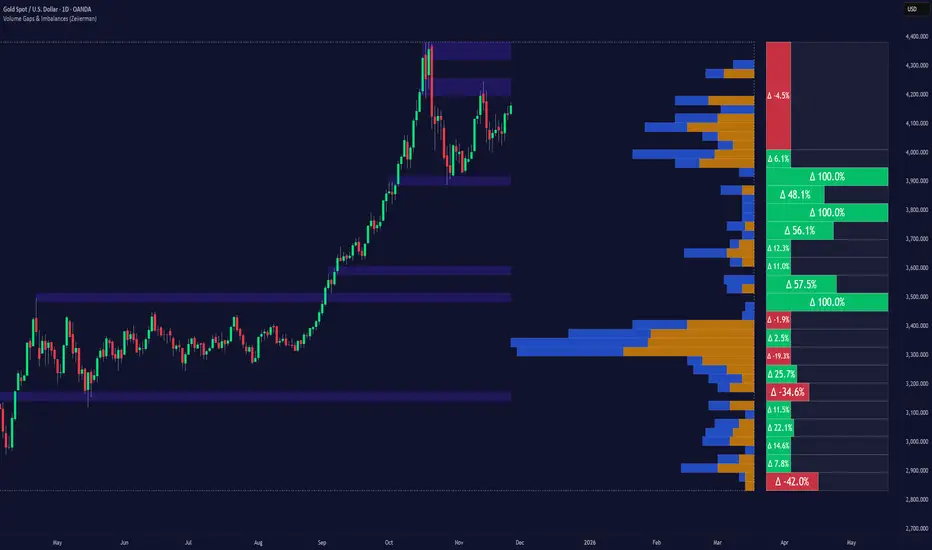
Tic Tac Toe Game [TradeDots]Feeling bored with trading?
Time to inject some fun into your decision-making process with our Tic Tac Toe Indicator!
The Tic Tac Toe game transforms your chart into a competitive playground where trading pairs face off in a classic game of Tic Tac Toe.
HOW TO PLAY
Our Tic Tac Toe game invites you to pit one trading pair against another directly on your chart. Choose the competitors and watch as they battle it out in a traditional grid setup.
Navigate to settings and select your competitor pair.
Choose who kicks off the game.
After the close of each new bar, the algorithm will utilize the closing prices of both symbols. These numbers feed into a random number generator which alternates the turns for placing marks on the grid.
The game progresses until one pair aligns three consecutive symbols and wins, or the board fills up. After that, the game resets every three bars, offering continual engagement during active market hours.
MANUAL PLAYING MODE
Currently, due to PineScript's limitations, a fully interactive manual mode is not supported, as all previous data will be lost with each new user input, preventing the replication of existing game states.
However, users can input a sequence at the start, guiding the placement of symbols throughout the game.
Stay tuned for future updates!

Custom Rotatable PinwheelCustom Rotatable Pinwheel – Art Generator (Fully Color-Configurable)
This visual indicator draws a rotating pinwheel using radial spokes. It's designed purely for artistic and decorative purposes — not for trading signals. Use it to create abstract, mandala-like effects by layering multiple instances with different rotation angles and color palettes.
Fully Customizable Spoke Colors
You can now define up to 8 custom spoke colors, which cycle across the pinwheel arms.
Optionally, enable "Use Single Color" to override all spokes with a single color.
This gives full creative control over your color palette and design aesthetic.
Controls:
Number of Spokes – Total number of radial arms
Rotation Offset (°) – Adjusts the starting angle, useful when layering multiple instances
Spin Speed – Controls how fast the pinwheel rotates with each bar
Inner / Outer Radius – Adjusts the spoke arm lengths
Transparency – Controls how visible the lines are
Use Single Color – Toggle between a single color or a full custom palette
Color 1–8 – Set your preferred spoke colors (used when single color is off)
Setup for a Clean Chart Canvas (No Price Bars or Gridlines)
To hide all default chart visuals and show only the pinwheel design:
Right-click chart → Settings
Symbol tab: Uncheck "Show Bars"
Scales tab: Uncheck "Price Scale" and "Time Scale"
Appearance tab:
Set background to black
Uncheck grid lines, watermark, etc.
Status Line and Events: Uncheck all
FunctionPatternDecompositionLibrary "FunctionPatternDecomposition"
Methods for decomposing price into common grid/matrix patterns.
series_to_array(source, length) Helper for converting series to array.
Parameters:
source : float, data series.
length : int, size.
Returns: float array.
smooth_data_2d(data, rate) Smooth data sample into 2d points.
Parameters:
data : float array, source data.
rate : float, default=0.25, the rate of smoothness to apply.
Returns: tuple with 2 float arrays.
thin_points(data_x, data_y, rate) Thin the number of points.
Parameters:
data_x : float array, points x value.
data_y : float array, points y value.
rate : float, default=2.0, minimum threshold rate of sample stdev to accept points.
Returns: tuple with 2 float arrays.
extract_point_direction(data_x, data_y) Extract the direction each point faces.
Parameters:
data_x : float array, points x value.
data_y : float array, points y value.
Returns: float array.
find_corners(data_x, data_y, rate) ...
Parameters:
data_x : float array, points x value.
data_y : float array, points y value.
rate : float, minimum threshold rate of data y stdev.
Returns: tuple with 2 float arrays.
grid_coordinates(data_x, data_y, m_size) transforms points data to a constrained sized matrix format.
Parameters:
data_x : float array, points x value.
data_y : float array, points y value.
m_size : int, default=10, size of the matrix.
Returns: flat 2d pseudo matrix.

Volume-Weighted Fibonacci PivotThis indicator automatically plots dynamic Fibonacci retracement and extension levels based on a volume-weighted pivot point within a user-defined lookback period or date range. It intelligently calculates a central "pivot" price biased toward high-volume bars, then draws symmetric levels both upward (extensions) and downward (retracements) for balanced confluence analysis.
How It Works (Technical Methodology)
Lookback Period Determination
Multiple filter modes control the data range used for calculations:
"Last X Bars": Fixed number of recent bars (default 400, max 4999).
"Manual Date": User-specified start date.
"Interactive (Chart)": Confirmed start date via input.
"None": Full available history (falls back to max bars).
Optionally, when using "Last X Bars", calculations can pull data from a higher/lower user-selected timeframe via request.security() for multi-timeframe alignment.
A dotted vertical line marks the start point in date-based modes.
Range and Pivot Calculation
Within the selected period:
Highest high and lowest low define the full price range.
Average volume is computed across the period.
Volume-Weighted Pivot: Average close price only from bars where volume > average volume (fallback to simple midpoint if no high-volume bars).
This creates a "smart" central pivot that leans toward areas of greater participation, often aligning with institutional activity.
Fibonacci Level Generation
User-configurable ratios (default: 0.236, 0.382, 0.5, 0.618, 0.786, 1.0, 1.272, 1.414, 1.618).
Levels are calculated symmetrically around the volume-weighted pivot:
Upward: Pivot + (Range × Ratio × Correction Factor) – teal/cyan shades.
Downward: Pivot - (Range × Ratio × Correction Factor) – red shades.
Correction Factor (default 0.5): Scales level spacing for tighter/wider grids without altering ratios.
Only the user-defined number of active lines (default 9) are drawn.
Visual Construction
Central Pivot Line: Thick yellow horizontal line with label showing exact price.
Up/Down Levels: Dashed lines extended into the future, labeled with ratio direction ("Up" or "Dn").
All objects redraw only on the last bar for performance, clearing previous drawings.
Multi-Timeframe Option
When enabled with "Last X Bars":
Pulls high/low/volume data from specified timeframe.
Aligns the pivot and levels to higher-timeframe structure while displaying on current chart – ideal for intraday traders seeking HTF confluence.
How to Use
This tool provides clean, volume-aware Fibonacci grids for identifying potential support/resistance, reversal zones, and targets.
Volume-Weighted Pivot: Often acts as a strong mean reversion level or fair value area.
Upward Levels (Teal): Potential resistance/extensions in bullish moves; watch for reactions on retests.
Downward Levels (Red): Potential support/retracements in bearish moves.
Confluence: High probability when price reacts at levels aligning with other tools (order blocks, pivots, volume profile).
Correction Factor: Lower values (<0.5) for tighter grids in ranging markets; higher (>0.5) for trending markets.
Multi-Timeframe Mode: Use on lower charts (e.g., 15m) with HTF input (e.g., 4H or Daily) to project major structure levels.
Common Setups:
Pullbacks to 0.618–0.786 zones for continuation entries.
Breaks beyond 1.0–1.618 for extension targets.
Reactions near pivot line for mean reversion trades.
Adjust ratios and active line count to match your preferred Fibonacci style (classic retracement vs. extensions).
Disclaimer
This indicator is a technical analysis tool and should be used in conjunction with other forms of analysis. Past performance does not guarantee future results. Always use proper risk management.
