Quantum Harmonic Oscillator Overlay🧪 Quantum Harmonic Oscillator Overlay
A visual model of price behavior using quantum harmonic oscillation principles
📜 Indicator Overview
The Quantum Harmonic Oscillator Overlay applies concepts from both classical physics (harmonic motion) and quantum mechanics (energy states) to model and visualize how price orbits around a central trend line. It overlays a Linear Regression line (representing the “mean position” or ground state of price) and calculates surrounding energy levels (σ-zones) akin to quantum shells that price can "jump" between.
This indicator is particularly useful for visualizing mean reversion, volatility compression/expansion, and momentum-driven price breakthroughs.
🧠 Core Concepts
Linear Regression Line (LSR): This is the calculated center of gravity or equilibrium path of price over a user-defined period. Think of it like the lowest energy state or central axis around which price vibrates.
Standard Deviation Zones (σ-levels):
1σ: The majority of normal price activity; within this range, price tends to fluctuate if in balance.
2σ: Indicates volatility or possible breakout pressure.
3σ: Represents extreme movement — a phase shift in energy, potentially leading to reversal or continuation with higher momentum.
Quantum Analogy: Just like in a quantum harmonic oscillator, particles (here, prices) move probabilistically between discrete energy states. The further the price moves from the center, the more "energy" (momentum, volume, volatility) is implied.
⚙️ Input Parameters
Setting Description
Linear Regression Length The number of bars used to calculate the regression trend (default 100). Affects the central path and responsiveness.
σ Multipliers (1σ, 2σ, 3σ) Determine how far each band is from the regression line. Adjusting these can highlight different price behaviors.
Show Energy Level Zones Toggle visibility of the colored bands around the regression line.
Show LSR Center Line Toggles visibility of the white Linear Regression line itself.
🎨 Visual Components
Color Zone Interpretation
✅ Green ±1σ Normal oscillation / mean reversion area. Ideal for range-bound strategies.
🟧 Orange ±2σ Warning zone; price may be gaining momentum or volatility.
🔴 Red ±3σ High-momentum state or anomaly. These regions may imply trend exhaustion, reversals, or breakouts.
White Line: The LSR — the average trajectory of the price movement.
Pink Dots: Appear when price exceeds Zone 3 (outside ±3σ) — a signal of extreme behavior or a possible regime shift.
📈 How to Use This Indicator
1. Detect Overextensions
When price touches or breaches the 3σ zone, it is likely overextended. This can be used to anticipate potential snapbacks or strong breakout trends.
2. Identify Mean Reversion Trades
If price exits the 2σ or 3σ zones and returns toward the center line, this signals a likely mean reversion setup.
3. Volatility Compression or Expansion
Flat zones between σ levels suggest calm markets; widening bands suggest expanding volatility.
4. Use with Confirmation Tools
Combine with momentum oscillators (MACD, RSI) or volume-based signals to confirm reversals or continuation outside Zone 3.
🔮 Philosophical Note
This indicator embodies the metaphor that the market behaves like a quantum oscillator — price particles exist in a probabilistic field and jump between discrete zones of volatility and energy. Tracking these transitions allows the trader to see price behavior as rhythmic, wave-like, and multidimensional rather than purely linear.
Recherche dans les scripts pour "oscillator"

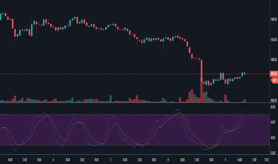
Divergence Detector [TradingFinder] RSI + MACD + AO Oscillator 🔵 Introduction
🟣 Understanding Divergence
As mentioned, divergence occurs in technical analysis when a stock's price behaves contrary to indicators on the price chart. Divergence can signify either a reversal of the stock's trend or a continuation of the previous trend correction.
Divergences can act as reversal patterns or continuation patterns. Moreover, divergences can be utilized to identify potential support and resistance levels.
For instance, when an indicator is trending upwards and positive, but the price is declining and trending downwards, divergence occurs. Divergence in a stock indicates trader indecision in buying and selling and warns traders to reconsider their decisions regarding buying or holding the stock.
Divergence aids analysts in identifying critical price points. In indicator divergences, it serves as a potent signal in the realm of technical analysis.
🟣 Types of Divergence
1.Regular Divergence
o Positive Regular Divergence (RD+)
o Negative Regular Divergence (RD-)
2.Hidden Divergence
o Positive Hidden Divergence (HD+)
o Negative Hidden Divergence (HD-)
3.Time Divergence
Key Note : This indicator is specifically designed to identify "Regular Divergence" only. Therefore, the following explanation pertains to this type of divergence.
🔵 Regular Divergence/Convergence
Regular Divergence(Convergence) occurs due to conflicting behavior between the indicator and the price chart, typically at the end of a trend. Recognizing Regular Divergence suggests an anticipation of a trend reversal or a pattern resembling a reversal.
🟣 Positive Regular Divergence (RD+)
In contrast to negative divergence, positive Regular Divergence occurs at the end of a downtrend and between two price lows. It manifests when the price forms a new low on the price chart, but the indicator fails to recognize it.
Positive Regular Divergence indicates strong buying pressure and weak selling pressure. Following the identification of positive divergence on the chart, one can anticipate a price increase for the examined stock.
🟣 Negative Regular Divergence (RD-)
This type of Regular Divergence emerges between two price highs during an uptrend. A new high is formed on the price chart, but the indicator fails to acknowledge it. This scenario indicates negative Regular Divergence.
The likelihood of a subsequent market downturn is high. Negative divergence signifies strong selling pressure and weak buying pressure, suggesting an unfavorable future for the stock.
🔵 How to use
By utilizing the "Fractal Period" input, you can specify your desired periods for identifying divergences.
Additionally, through the "Divergence Detect Method" feature, you can choose which oscillators (MACD, RSI, or AO) to base divergence identification on.
Divergence in MACD Oscillator :
Divergence in the MACD indicator occurs when the price chart and the MACD line form a noticeable opposing pattern, meaning the price moves contrary to the MACD line. In this scenario, one expects a reversal in price direction.
Divergence in RSI Oscillator :
If divergence occurs during a downtrend on the price chart (two consecutive lows, with the second low being lower) and on the corresponding RSI point (two consecutive lows, with the second low being higher), it signifies positive Regular Divergence and implies a buying signal.
Conversely, if divergence occurs during an uptrend on the price chart (two consecutive highs, with the second high being higher) and on the corresponding RSI point (two consecutive highs, with the second high being lower), it indicates negative Regular Divergence, signaling a selling opportunity.
Divergence in AO Oscillator :
The AO indicator calculates histograms similar to the AO base. It calculates the difference between the simple moving averages of 5 and 34 periods based on the median of each bar. Then, it plots the bars based on the difference.
It then compares the histograms to detect peaks and troughs in the AO histograms and compares the identified peaks and troughs to the price. Whenever divergence is detected, it plots lines and arrows.
🔵 Table
The table contains information on the functional features of this oscillator that you can utilize. Four categories of information are presented in the table: "Exist," "Consecutive," "Divergence Quality," and "Change Phase Indicator."
Exist :
If divergence exists, you'll see "+" in this row.
Consecutive :
Divergences may occur consecutively. If same-type divergences form within short intervals, you can observe the count in this row.
Divergence Quality : Based on the number of consecutive divergences, their quality can be evaluated. If one divergence exists, its quality is considered "Normal." If two divergences exist, the quality is "Good," and if three or more divergences exist, the quality is considered "Strong."
Change Phase Indicator : If a phase change occurs between two oscillation peaks formed based on divergence, this change is identified and displayed in this row.

Rolling VWAP OscillatorTL;DR - TradingView's Rolling VWAP as centered oscillator
I really like TradingView's rolling VWAP (Rolling Volume-Weighted Average Price - RVWAP) indicator. But I also like clean charts that's why I'm mainly using indicators which are not displayed on the chart. Instead of simply moving the RVWAP to another pane I turned it into a centered oscillator. This allows me checking the RVWAP while having my chart clean.
You can find the oroginal RVWAP here .
Creds to TradingView for creating this indicator 👍
* I also added a fourth deviation band, gradient colors and the option to switch between candles and lines.

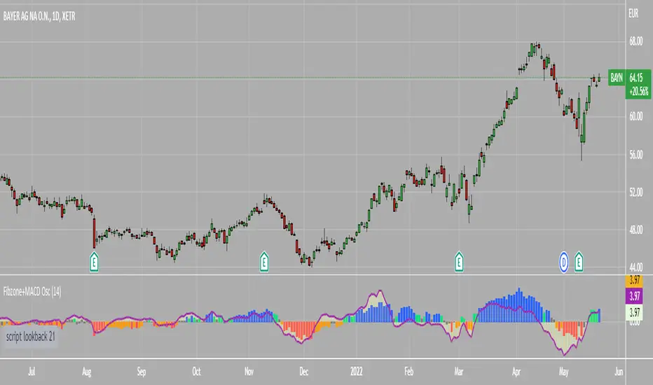
Fibonacci Zone Oscillator With MACD HistogramThe columns
After I found a way to calculate a price as a percent of the middle line of the KeltCOG Channel in the KCGmut indicator (published), I got the idea to use the same trick in the Fbonacci Zone Channel (also published), thus creating an oscillator.
I plot the percent’s as columns with the color of the KeltCOG Channel. Because the channels I created and published (i.e. Fibonacci Zone, Donchian Fibonacci Trading Tool, Keltner Fibzones, and KeltCOG) all use Fibonacci zones, this indicator also reports the position of the close in their zones.
Strategy and Use:
Blue column: Close in uptrend area, 4 supports, 0 resistance, ready to rally up.
Green column: Close in buyers area, 3 supports, 1 resistance, looking up.
Gray column: Close in center area 2 supports, 2 resistances, undecided.
Yellow column: Close in sellers area 1 support, 3 resistances, looking down.
Red column: Close in downtrend area, 0 support, 4 resistances, ready to rally down.
I use this indicator in a layout with three timeframes which I use for stock picking, I pick all stocks with a blue column in every timeframe, the indicator is so clear that I can flip through the 50 charts of my universe of high liquid European blue chips in 15 minutes to make a list of these stocks.
Because I use it in conjunction with KeltCOG I also gave it a ‘script sets lookback’ option which can be checked with a feedback label and switched off in the inputs.
The MACD histogram
I admire the MACD because it is spot on when predicting tops and bottoms. It is also the most sexy indictor in TA. Actually just the histogram is needed, so I don’t show the macd-line and the signal line. I use the same lookback for the slow-ma as for the columns, set the fast-ma to half and the signal-line to a third of the general lookback. Therefore I gave the lookback a minimum value of 6, so the signal gets at least a lookback of 2.
The histogram is plotted three times, first as a whitish area to provide a background, then the colums of the Fibzone Oscillator are plotted, then the histogram as a purple line, which contrasts nicely and then as a hardly visible brown histogram.
The input settings give the option to show columns and histogram separate or together.
Strategy and use:
I think about the columns as showing a ‘longer term chosen momentum’ and about the histogram as a ‘short term power momentum’. I use it as additional information.
Enjoy, Eykpunter.
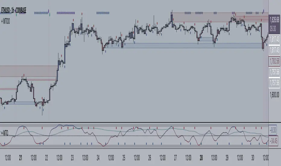
+ WaveTrend Oscillator OverlayAn overlay version of pertinent signals from my version of LazyBear's Wavetrend Oscillator.
Shows momentum of long period WTO as either background colors or symbols.
Shows continuation and reversal trade signals.
If Secondary WTO is above the center line (momentum is long), then symbols print across the top of the chart when the primary (faster) WTO comes into "oversold," a number associated with a horizontal line on the off-chart indicator. This number is selectable via a drop-down menu. Same thing for bearish momentum.
Conversely, reversal signals are printed along the bottom when conditions are met. Ex: if the Secondary WTO is showing momentum is bullish, then symbols will print along the bottom when the primary WTO is at "overbought" (or whatever number you deem overbought--again, via a similar drop-down menu).
Also, symbols are printed above and below candles for when the moving average of the primary WTO is crossed.
You could use these for taking profits, exiting a trade, or entering a trade.
Includes a moving average that is an average of the 200 EMA, SMA and Kijun.
Alerts.
Enjoy.
//p.s. I recommend using this in conjunction with my "+ Wavetrend Oscillator" at least starting out. Helps to have a visual
//reference when picking reversal and continuation numbers.
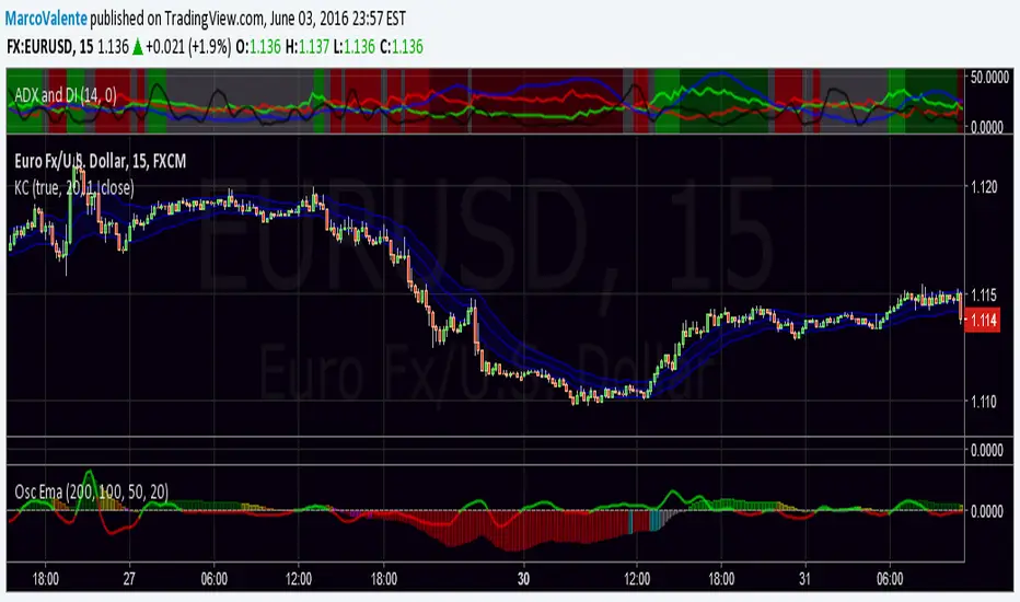
[jav] Mountain Oscillator
Introducing the Mountain Oscillator. Why not trading while admiring the scenery?
The main oscillator line is the black silhouette of the mountains, and each element of the landscape can be seen as a support or resistance - even the mountains far in the horizon, the misty band in the middle and the -1, 0 and 1 lines. (Well, almost every element... the sun is just for fun).
Equalling the heights of the mountains that are far away, or reaching the snow zone, are possible signs of an uptrend ending. On the other hand, stepping into a river is a clear sign of a reversal to the upside soon.
Strong uptrends are evidenced by significant portions of the mountain above the misty zone and/or the 0 line.
By default, the sky turns red/blue/dark gray depending on the trading hours. This option can be unchecked.
Calculations and usage :
The script is based on a modified version of Bollinger Bands. Bandwidth is calculated quite differently from the usual Bollinger indicator (not with the built-in stdev function). There is no need to input a multiplier factor, such as that used in BB - the script calculates it from 'Length' using a custom formula.
The 3 user inputs 'Length' ares recommended to be kept at 200, 100 and 50 period. In that way, the misty area in the landscape corresponds to price crossing EMAs of 50 and 100, and the zero line to EMA 200.
The different colors of the mountain and the horizon represent the Bollinger Bands corresponding to the mentioned periods of 50 and 100, whereas limits of -1 and +1 are those from the 'Length' parameter.
You will find that my coding skills are rudimentary, so any comment/suggestion to improve the script is welcome.
Credits
@everget for the 'Fancy Shapes' script which was used as a reference to draw the sun.

CMO (Chande Momentum Oscillator)Hi
Let me introduce my CMO (Chande Momentum Oscillator) script.
This indicator plots Chandre Momentum Oscillator. This indicator was
developed by Tushar Chande. A scientist, an inventor, and a respected
trading system developer, Mr. Chande developed the CMO to capture what
he calls "pure momentum". For more definitive information on the CMO and
other indicators we recommend the book The New Technical Trader by Tushar
Chande and Stanley Kroll.
The CMO is closely related to, yet unique from, other momentum oriented
indicators such as Relative Strength Index, Stochastic, Rate-of-Change,
etc. It is most closely related to Welles Wilder`s RSI, yet it differs
in several ways:
- It uses data for both up days and down days in the numerator, thereby
directly measuring momentum;
- The calculations are applied on unsmoothed data. Therefore, short-term
extreme movements in price are not hidden. Once calculated, smoothing
can be applied to the CMO, if desired;
- The scale is bounded between +100 and -100, thereby allowing you to
clearly see changes in net momentum using the 0 level. The bounded scale
also allows you to conveniently compare values across different securities.

David Varadi Intermediate OscillatorThe David Varadi Intermediate Oscillator (DVI) is a composite momentum oscillator designed to generate trading signals based on two key factors: the magnitude of returns over different time windows and the stretch, which measures the relative number of up versus down days. By combining these factors, the DVI aims to provide a reliable and objective assessment of market trends and momentum.
Methodology:
To calculate the DVI, a specific formula is applied. The magnitude component involves averaging smoothed returns over various lengths, weighted according to user-defined parameters. This calculation helps determine the magnitude of price changes. The stretch component follows a similar process, averaging smoothed returns over different lengths to gauge market momentum. Users have the flexibility to adjust the weights and lengths to suit their trading preferences and styles.
Utility:
The DVI offers versatility in its applications. It can be used for both momentum trading and trend analysis due to its smooth and consistent signals. Unlike some other oscillators, the DVI provides longer and uncorrelated signals, allowing traders to effectively combine trend-following and mean-reversion strategies. For example, the DVI is adept at identifying overbought levels above the 200-day moving average, serving as a useful tool for determining exit points during price strength and even potential shorting opportunities. Traders can develop simple trading systems based on the DVI, buying above the 200-day moving average and selling when the DVI exceeds a specified threshold. Conversely, they can consider short positions below the 200-day moving average and cover when the DVI falls below a specific threshold. The DVI's objective approach to analyzing market momentum makes it a valuable resource for traders seeking to identify trading opportunities.
Key Features:
Bar coloring: based on Trend, Extremeties or Reversions
Reversions: Potential reversal points marked with triangles above\below oscillator
Extremity Hues: Highlighting oxcillator reaching traditional OB\OS levels
Example Charts:

Rotational Gravity OscillatorMade using elements from two Cheatcountry scripts:
Includes a Bollinger Band for bounds that forms a trend follower based on the 0 point.
Includes CheatCountry color code signals, different color scheme. Bright colors are strong signals, ark are weak, green bull, red bear, the basics.
Switches for Bollinger Band color codes, which can actually be useful signals.
This oscillator can be used for divergences, trends, signal strength, confirmation, volatility readings, you name it.
It is a comparative oscillator, that compares adaptively smoothed, weighted modified Change of Gravity oscillators between 2 symbols and multiple lengths to determine directional momentum as one asset compares to another.
The default uses the Crypto TOTAL market cap to help trade cryptocurrencies. You will notice that BTC will give sell signals in uptrends at times. That is because it is being compared to an index of the total Crypto market cap, and since alt-coins move faster, BTC will lag behind this index.
Give CheatCountry a follow, hes one of the MVPs of Tradingview Pinescripters, constantly giving us access to novel new concepts as they are published by professionals.

Cumulative Volume OscillatorCVO: Cumulative Volume Oscillator allows you to choose between 3 types of oscillators based on volume indicators:
-OBV (On Balance Volume)
-CVD (Cumulative Volume Delta)
-PVT (Price Volume Trend)
Being a volume based oscillator this indicator allows for the detection of divergences between price action and volume, ideal for predicting reversals.
As an oscillator you can choose the length of the fast & slow EMAs, and a signal line is provided for trend following.

Karobein OscillatorDeveloped by Emily Karobein, the Karobein oscillator is an oscillator that aim to rescale smoothed values with more reactivity in a range of (0,1)
Calculation
The scaling method is similar to the one used in a kalman filter for the kalman gain.
We first average the up/downs x, those calculations are similar to the ones used for calculating the average gain/loss in the relative strength index.
a = ema(src < src ? x : 0,length)
b = ema(src > src ? x : 0,length)
where src is a exponential moving average of length period and x is src/src in the standard calculations, but anything else can be used as long as x > 0 .
Then we rescale the results.
c = x/(x + b)
d = 2*(x/(x + c*a)) - 1
How To Use
It is better to use centerline-cross/breakouts/signal line.
In general when we use something smooth as input in oscillators, breakouts are better than reversals, you can see this with the stochastic and rsi.
So a simple approach could be buying when crossing over 0.8 and selling when crossing under 0.2.
Here is the balance of a strategy using those conditions, length = 50 .
20 trades have been mades since the 29 oct we made 341 pips with eur/usd, of course this backtest was made during good trends period,
this result is not representative of how the strategy work with other conditions/markets.
For any questions/suggestions feel free to contact me

oscillatore EMAOscillator make from 4 ema, Columns give us the trend and signal line can be use to find divergenge or as buy/sell trigger. Colors changes to indicate the relation between price and Ema
Volability is calculate using deviation st.
DecisionPoint Volume Swenlin Trading Oscillator [LazyBear]This is the volume version of "DecisionPoint Breadth Swenlin Trading Oscillator"
DecisionPoint Swenlin Trading Oscillator can be used to identify short-term tops and bottoms. You can read about the interpretation of the signals (& gotchas) in the link below.
I have added support for NYSE / NASD / AMEX and also a combined mode. You can specify custom advancing/declining volume symbols too.
More Info:
DBSTO:
Article: stockcharts.com
List of my public indicators: bit.ly
List of my app-store indicators: blog.tradingview.com
Having both Swenlin Breadth and Volume oscillators help spot the divergences quickly:

Overextension Oscillator [by DanielM]The Overextension Oscillator is an indicator that detects when a market move has extended significantly beyond its typical range, signaling potential areas for a correction or reversal. Unlike traditional oscillators that rely on fixed overbought/oversold levels, this tool dynamically adjusts its thresholds based on historical swing high and swing low movements.
By analyzing all swing points on the chart, the indicator determines the expected range of price movements and identifies when the price extends beyond normal levels. Since every asset has different price behavior and volatility, swing lengths may vary from asset to asset, ensuring that overextension is measured relative to each market's historical price behavior.
How It Works
1️⃣ Swing Detection & Data Collection
The indicator scans all available swing highs and swing lows on the chart to gather a complete dataset of past price fluctuations.
It records the percentage differences between swings to determine how much price typically moves in a given market.
2️⃣ Overextension Calculation
Using the stored swing data, the indicator calculates:
Average Swing Difference – Measures the average percentage difference between swings.
Average Move Percentage – Determines the typical magnitude of price moves within a trend cycle.
These values are used to create dynamic overextension thresholds that adjust based on historical data.
3️⃣ Price Distance & Overextension Measurement
The indicator calculates the distance between the current price and the closest historical swing point. If this distance exceeds the predefined threshold based on past swings, the move is considered overextended. The greater the deviation, the higher the probability of a pullback or short-term reversal.
4️⃣ Buy/Sell Signal Generation
A Buy signal is generated when the price has dropped below an overextended threshold relative to a past swing low.
A Sell signal is generated when the price has risen beyond an overextended threshold relative to a past swing high.
These signals indicate that the price has reached a level where it historically tends to slow down or reverse.

HMA Slope OscillatorA Hull Moving Average (HMA) slope oscillator. It uses a HMA slope to identify up/down trends. Usage is simple: adjust the HMA and signal length according to your needs. Long orders start when the bar changes from under (the zero line) to over the zero line. You can also spot "early" long entries when the bar moves close to the zero line. Short orders should be placed when a red bar appears after blue bars (top of the mountain).
"Play" with the length to find the best settings for your trading strategy.
** I have not added alerts. If you need alerts just let me know and I will be happy to update this indicator.

Weighted Harrell-Davis Quantile Estimator with AD Oscillatorxel_arjona
Licensing:
This work is licensed under a Attribution-NonCommercial-ShareAlike 4.0 International Copyright (c) 2021 ( CC BY-NC-SA 4.0)
Copyright's & Mentions:
The Gamma Functions & Beta Probability Density Functions C# implementations by the Math.NET Numerics, part of the Math.NET Project.
The Regularized Incomplete (Left) Beta Function C# implementation by the SAMTools, htslib project.
The Weighted Harrell-Davis Quantile estimator; C# & R implementations by Andrey Akinshin.
External PineScript code, methods, support & consultancy by @PineCoders staff with special mention for:
+ "ma sorter ('sort by array' example)- JD" by @Duyck.
+ Porting, mods, compilation and debugging for this script by @XeL_Arjona for the TradingView's @PineCoders community.
I made it an oscillator. Features include normalization, line display, and smoothing. :DDD Enjoy!
(Ive been wanting to do this for a while but I wanted to make the library first but you know what this was fun so there you go its here now)

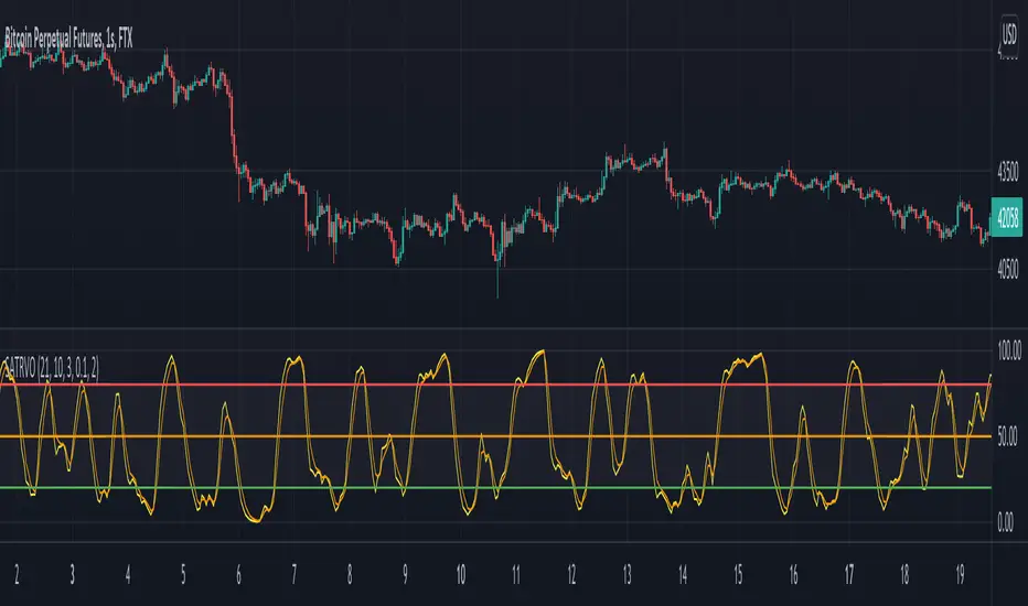
Stochastic ATR Volatility OscillatorNOTES: As x, k and d use;
21-10-3 for 1 Hour candles
5-4-2 for 4 Hour candles
21-21-3 for 1 Day candles
Yellow plot is the main oscillator. Orange plot, and hlines at 20, 50 and 80 can be used as signal lines.
I personally use hlines as the signal in 1H as it's the best timeframe for the indicator.
If you are in a long position, sell when yellow plot crosses 80 or 50 line downwards;
and buy when the line crosses 20, 50 or 75 upwards while you are not in a trade.
DiNapoli Preferred Stochastic Oscillator [ChuckBanger]In the late 1950s, George Lane developed stochastics, an indicator that measures the relationship between an issue's closing price and its price range over a predetermined period of time. This is Joe DiNapoli version of stochastic oscillator. Use it as you wold use a regular stochastic indicator.
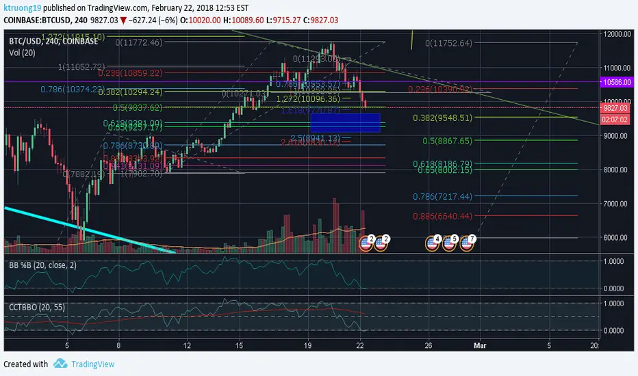
CCT Bollinger Band Oscillator - BB %B UpdateEdit of LazyBear's CCT Bollinger Band Oscillator. Includes changing the scale from 0-100 to 0-1, default length to 20 and line width to 1 to further match BB %B and address some middle line inconsistencies at certain zoom levels
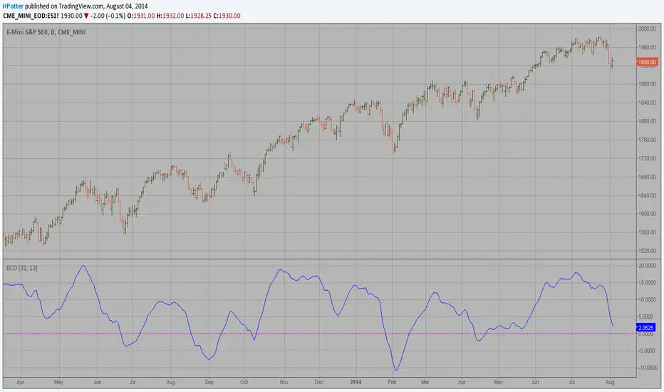
ECO (Blau`s Ergodic Candlestick Oscillator) We call this one the ECO for short, but it will be listed on the indicator list
at W. Blau’s Ergodic Candlestick Oscillator. The ECO is a momentum indicator.
It is based on candlestick bars, and takes into account the size and direction
of the candlestick "body". We have found it to be a very good momentum indicator,
and especially smooth, because it is unaffected by gaps in price, unlike many other
momentum indicators.
We like to use this indicator as an additional trend confirmation tool, or as an
alternate trend definition tool, in place of a weekly indicator. The simplest way
of using the indicator is simply to define the trend based on which side of the "0"
line the indicator is located on. If the indicator is above "0", then the trend is up.
If the indicator is below "0" then the trend is down. You can add an additional
qualifier by noting the "slope" of the indicator, and the crossing points of the slow
and fast lines. Some like to use the slope alone to define trend direction. If the
lines are sloping upward, the trend is up. Alternately, if the lines are sloping
downward, the trend is down. In this view, the point where the lines "cross" is the
point where the trend changes.
When the ECO is below the "0" line, the trend is down, and we are qualified only to
sell on new short signals from the Hi-Lo Activator. In other words, when the ECO is
above 0, we are not allowed to take short signals, and when the ECO is below 0, we
are not allowed to take long signals.
TheLark: Directional Movement Index OscillatorA modified DMI, This turns the standard DMI into an Oscillator. The DMI cross signal is the same, but as an OSC you get the added benefits or finding divergences, etc. The added WIlder's Average Line (blue) can help you see if a short term trend is getting less interesting.

OBV & AD Oscillators with Dual Smoothing OptionsOn Balance Volume and Accumulation/Distribution
Overlaid into 1 and then some,
Now it is an oscillator!
3 customizable moving average types
- Ehlers Deviation Scaled Moving Average
- Volatility Dynamic Moving Average
- Simple Moving Average
Each with customizable periods
And with the ability to overlay a second set too
Default Settings have a longer period MA of 377 using Ehlers DSMA to better capture the standard view of OBV and A/D.
An extra overlay of a shorter period using a Volatility DMA uses Average True Range with its own custom settings, seeks to act more as an RSI

SynchroTrend Oscillator (STO) [PhenLabs]📊 SynchroTrend Oscillator
Version: PineScript™ v5
📌 Description
The SynchroTrend Oscillator (STO) is a multi-timeframe synchronization tool that combines trend information from three distinct timeframes into a single, easy-to-interpret oscillator ranging from -100 to +100.
This indicator solves the common problem of having to analyze multiple timeframe charts separately by consolidating trend direction and strength across different time horizons. The STO helps traders identify when markets are truly synchronized across timeframes, potentially indicating stronger trend conditions and higher probability trading opportunities.
Using either Moving Average crossovers or RSI analysis as the trend definition metric, the STO provides a comprehensive view of market structure that adapts to various trading strategies and market conditions.
🚀 Points of Innovation
Triple-timeframe synchronization in a single view eliminates chart switching
Dual trend detection methods (MA vs Price or RSI) for flexibility across different markets
Dynamic color intensity that automatically increases with signal strength
Scaled oscillator format (-100 to +100) for intuitive trend strength interpretation
Customizable signal thresholds to match your risk tolerance and trading style
Visual alerts when markets reach full synchronization states
🔧 Core Components
Trend Scoring System: Calculates a binary score (+1, -1, or 0) for each timeframe based on selected metrics, providing clear trend direction
Multi-Timeframe Synchronization: Combines and scales trend scores from all three timeframes into a single oscillator
Dynamic Visualization: Adjusts color transparency based on signal strength, creating an intuitive visual guide
Threshold System: Provides customizable levels for identifying potentially significant trading opportunities
🔥 Key Features
Triple Timeframe Analysis: Synchronizes three user-defined timeframes (default: 60min, 15min, 5min) into one view
Dual Trend Detection Methods: Choose between Moving Average vs Price or RSI-based trend determination
Adjustable Signal Smoothing: Apply EMA, SMA, or no smoothing to the oscillator output for your preferred signal responsiveness
Dynamic Color Intensity: Colors become more vibrant as signal strength increases, helping identify strongest setups
Customizable Thresholds: Set your own buy/sell threshold levels to match your trading strategy
Comprehensive Alerts: Six different alert conditions for crossing thresholds, zero line, and full synchronization states
🎨 Visualization
Oscillator Line: The main line showing the synchronized trend value from -100 to +100
Dynamic Fill: Area between oscillator and zero line changes transparency based on signal strength
Threshold Lines: Optional dotted lines indicating buy/sell thresholds for visual reference
Color Coding: Green for bullish synchronization, red for bearish synchronization
📖 Usage Guidelines
Timeframe Settings
Timeframe 1: Default: 60 (1 hour) - Primary higher timeframe for trend definition
Timeframe 2: Default: 15 (15 minutes) - Intermediate timeframe for trend definition
Timeframe 3: Default: 5 (5 minutes) - Lower timeframe for trend definition
Trend Calculation Settings
Trend Definition Metric: Default: “MA vs Price” - Method used to determine trend on each timeframe
MA Type: Default: EMA - Moving Average type when using MA vs Price method
MA Length: Default: 21 - Moving Average period when using MA vs Price method
RSI Length: Default: 14 - RSI period when using RSI method
RSI Source: Default: close - Price data source for RSI calculation
Oscillator Settings
Smoothing Type: Default: SMA - Applies smoothing to the final oscillator
Smoothing Length: Default: 5 - Period for the smoothing function
Visual & Threshold Settings
Up/Down Colors: Customize colors for bullish and bearish signals
Transparency Range: Control how transparency changes with signal strength
Line Width: Adjust oscillator line thickness
Buy/Sell Thresholds: Set levels for potential entry/exit signals
✅ Best Use Cases
Trend confirmation across multiple timeframes
Finding high-probability entry points when all timeframes align
Early detection of potential trend reversals
Filtering trade signals from other indicators
Market structure analysis
Identifying potential divergences between timeframes
⚠️ Limitations
Like all indicators, can produce false signals during choppy or ranging markets
Works best in trending market conditions
Should not be used in isolation for trading decisions
Past performance is not indicative of future results
May require different settings for different markets or instruments
💡 What Makes This Unique
Combines three timeframes in a single visualization without requiring multiple chart windows
Dynamic transparency feature that automatically emphasizes stronger signals
Flexible trend definition methods suitable for different market conditions
Visual system that makes multi-timeframe analysis intuitive and accessible
🔬 How It Works
1. Trend Evaluation:
For each timeframe, the indicator calculates a trend score (+1, -1, or 0) using either:
MA vs Price: Comparing close price to a moving average
RSI: Determining if RSI is above or below 50
2. Score Aggregation:
The three trend scores are combined and then scaled to a range of -100 to +100
A value of +100 indicates all timeframes show bullish conditions
A value of -100 indicates all timeframes show bearish conditions
Values in between indicate varying degrees of alignment
3. Signal Processing:
The raw oscillator value can be smoothed using EMA, SMA, or left unsmoothed
The final value determines line color, fill color, and transparency settings
Threshold levels are applied to identify potential trading opportunities
💡 Note:
The SynchroTrend Oscillator is most effective when used as part of a comprehensive trading strategy that includes proper risk management techniques. For best results, consider using the oscillator in conjunction with support/resistance levels, price action analysis, and other complementary indicators that align with your trading style.