Pair Cointegration & Static Beta Analyzer (v6)Pair Cointegration & Static Beta Analyzer (v6)
This indicator evaluates whether two instruments exhibit statistical properties consistent with cointegration and tradable mean reversion.
It uses long-term beta estimation, spread standardization, AR(1) dynamics, drift stability, tail distribution analysis, and a multi-factor scoring model.
1. Static Beta and Spread Construction
A long-horizon static beta is estimated using covariance and variance of log-returns.
This beta does not update on every bar and is used throughout the entire model.
Beta = Cov(r1, r2) / Var(r2)
Spread = PriceA - Beta * PriceB
This “frozen” beta provides structural stability and avoids rolling noise in spread construction.
2. Correlation Check
Log-price correlation ensures the instruments move together over time.
Correlation ≥ 0.85 is required before deeper cointegration diagnostics are considered meaningful.
3. Z-Score Normalization and Distribution Behavior
The spread is standardized:
Z = (Spread - MA(Spread)) / Std(Spread)
The following statistical properties are examined:
Z-Mean: Should be close to zero in a stationary process
Z-Variance: Measures amplitude of deviations
Tail Probability: Frequency of |Z| being larger than a threshold (e.g. 2)
These metrics reveal whether the spread behaves like a mean-reverting equilibrium.
4. Mean Drift Stability
A rolling mean of the spread is examined.
If the rolling mean drifts excessively, the spread may not represent a stable long-term equilibrium.
A normalized drift ratio is used:
Mean Drift Ratio = Range( RollingMean(Spread) ) / Std(Spread)
Low drift indicates stable long-run equilibrium behavior.
5. AR(1) Dynamics and Half-Life
An AR(1) model approximates mean reversion:
Spread(t) = Phi * Spread(t-1) + error
Mean reversion requires:
0 < Phi < 1
Half-life of reversion:
Half-life = -ln(2) / ln(Phi)
Valid half-life for 10-minute bars typically falls between 3 and 80 bars.
6. Composite Scoring Model (0–100)
A multi-factor weighted scoring system is applied:
Component Score
Correlation 0–20
Z-Mean 0–15
Z-Variance 0–10
Tail Probability 0–10
Mean Drift 0–15
AR(1) Phi 0–15
Half-Life 0–15
Score interpretation:
70–100: Strong Cointegration Quality
40–70: Moderate
0–40: Weak
A pair is classified as cointegrated when:
Total Score ≥ Threshold (default = 70)
7. Main Cointegration Panel
Displays:
Static beta
Log-price correlation
Z-Mean, Z-Variance, Tail Probability
Drift Ratio
AR(1) Phi and Half-life
Composite score
Overall cointegration assessment
8. Beta Hedge Position Sizing (Average-Price Based)
To provide a more stable hedge ratio, hedge sizing is computed using average prices, not instantaneous prices:
AvgPriceA = SMA(PriceA, N)
AvgPriceB = SMA(PriceB, N)
Required B per 1 A = Beta * (AvgPriceA / AvgPriceB)
Using averaged prices results in a smoother, more reliable hedge ratio, reducing noise from bar-to-bar volatility.
The panel displays:
Required B security for 1 A security (average)
This represents the beta-neutral quantity of B required to hedge one unit of A.
Overview of Classical Stationarity & Cointegration Methods
The principal econometric tools commonly used in assessing stationarity and cointegration include:
Augmented Dickey–Fuller (ADF) Test
Phillips–Perron (PP) Test
KPSS Test
Engle–Granger Cointegration Test
Phillips–Ouliaris Cointegration Test
Johansen Cointegration Test
Since these procedures rely on regression residuals, matrix operations, and distribution-based critical values that are not supported in TradingView Pine Script, a practical multi-criteria scoring approach is employed instead. This framework leverages metrics that are fully computable in Pine and offers an operational proxy for evaluating cointegration-like behavior under platform constraints.
References
Engle & Granger (1987), Co-integration and Error Correction
Poterba & Summers (1988), Mean Reversion in Stock Prices
Vidyamurthy (2004), Pairs Trading
Explanation structured with assistance from OpenAI’s ChatGPT
Regards.
Tail

VIX - SKEW DivergenceThe CBOE VIX is a well-known index representing market expectations for volatility over the next 30 days.
The CBOE SKEW is an index reflecting the perceived tail risk over the next 30 days.
When the SKEW rises over a certain level (~140/150), that means investors are hedging their exposure with options, because they are worried about an incoming market crash or a "black swan". If that happens when the VIX is very low and apparently there is no uncertainty, this can warn of a sudden change in direction of the market. You will see for yourself that an increasing divergence often anticipates a sharp fall of leading stock indexes, usually within two to four months.
This is probably not very relevant for the short-term trader but mid/long-term traders and market analysts may find it useful to clearly visualize the extent of the distance between the VIX and the SKEW. For that reason, I wrote this highly customizable script with which you can plot the two indexes and fill the space within them with a color gradient to highlight the maximum and minimum divergence. Additionally, you can fill the beneath VIX area with four different colors. It is also possible to plot the divergence value itself, so if you want you can draw trendlines and support/resistance levels on it.
Please note that the divergence per se doesn't predict anything and it's meant to be used synergistically with other technical analysis tools.
More informations here:
www.cboe.com
www.cboe.com

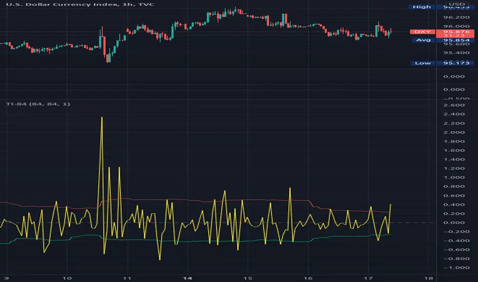
Tail Indicator - 84Like a old faithful calculator the Tail Indicator - 84 will calculate the tail strength of the forces that drag the price against its momentum.
ps:.. the pun is totally intended. :)