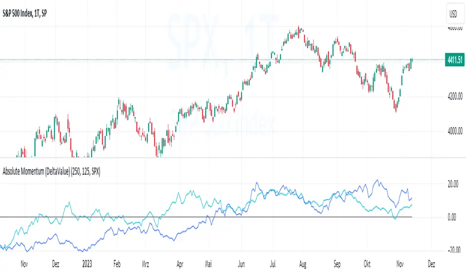
Absolute Momentum (Time Series Momentum)Absolute momentum , also known as time series momentum , focuses on the trend of an asset's own past performance to predict its future performance. It involves analyzing an asset's own historical performance, rather than comparing it to other assets.
The strategy determines whether an asset's price is exhibiting an upward (positive momentum) or downward (negative momentum) trend by assessing the asset's return over a given period (standard look-back period: 12 months or approximately 250 trading days). Some studies recommend calculating momentum by deducting the corresponding Treasury bill rate from the measured performance.
Absolute Momentum Indicator
The Absolute Momentum Indicator displays the rolling 12-month performance (measured over 250 trading days) and plots it against a horizontal line representing 0%. If the indicator crosses above this line, it signifies positive absolute momentum, and conversely, crossing below indicates negative momentum. An additional, optional look-back period input field can be accessed through the settings.
Hint: This indicator is a simplified version, as some academic approaches measure absolute momentum by subtracting risk-free rates from the 12-month performance. However, even with higher rates, the values will still remain close to the 0% line.
Benefits of Absolute Momentum
Absolute momentum, which should not be confused with relative momentum or the momentum indicator, serves as a timing instrument for both individual assets and entire markets.
Gary Antonacci , a key contributor to the absolute momentum strategy (find study below), emphasizes its effectiveness in multi-asset portfolios and its importance in long-only investing. This is particularly evident in a) reducing downside volatility and b) mitigating behavioral biases.
Moskowitz, Ooi, and Pedersen document significant 'time series momentum' across various asset classes, including equity index, currency, commodity, and bond futures, in 58 liquid instruments (find study below). There's a notable persistence in returns ranging from one to 12 months, which tends to partially reverse over longer periods. This pattern aligns with sentiment theories suggesting initial under-reaction followed by delayed over-reaction.
Despite its surprising ease of implementation, the academic community has successfully measured the effects of absolute momentum across decades and in every major asset class, including stocks, bonds, commodities, and foreign exchange (FX).
Strategies for Implementing Absolute Momentum:
To Buy a Stock:
Select a Look-Back Period: Choose a historical period to analyze the stock's performance. A common period is 12 months, but this can vary based on your investment strategy.
Calculate Excess Return: Determine the stock's excess return over this period. You can also assume a risk-free rate of "0" to simplify the process.
Evaluate Momentum:
If the excess return is positive, it indicates positive absolute momentum. This suggests the stock is in an upward trend and could be a good buying opportunity.
If the excess return is negative, it suggests negative momentum, and you might want to delay buying.
Consider further conditions: Align your decision with broader market trends, economic indicators, or fundamental analysis, for additional context.
To Sell a Stock You Own:
Regularly Monitor Performance: Use the same look-back period as for buying (e.g., 12 months) to regularly assess the stock's performance.
Check for Negative Momentum: Calculate the excess return for the look-back period. Again, you can assume a risk-free rate of "0" to simplify the process. If the stock shows negative momentum, it might be time to consider selling.
Consider further conditions:Align your decision with broader market trends, economic indicators, or fundamental analysis, for additional context.
Important note: Note: Entering a position (i.e., buying) based on positive absolute momentum doesn't necessarily mean you must sell it if it later exhibits negative absolute momentum. You can initiate a position using positive absolute momentum as an entry indicator and then continue holding it based on other criteria, such as fundamental analysis.
General Tips:
Reassessment Frequency: Decide how often you will reassess the momentum (monthly, quarterly, etc.).
Remember, while absolute momentum provides a systematic approach, it's recommendable to consider it as part of a broader investment strategy that includes diversification, risk management, fundamental analysis, etc.
Relevant Capital Market Studies:
Antonacci, Gary. "Absolute momentum: A simple rule-based strategy and universal trend-following overlay." Available at SSRN 2244633 (2013)
Moskowitz, Tobias J., Yao Hua Ooi, and Lasse Heje Pedersen. "Time series momentum." Journal of financial economics 104.2 (2012): 228-250
Recherche dans les scripts pour "12月4号是什么星座"
S&P 500 Quandl Data & RatiosTradingView has a little-known integration that allows you to pull in 3rd party data-sets from Nasdaq Data Link, also known as Quandl. Today, I am open-sourcing for the community an indicator that uses the Quandl integration to pull in historical data and ratios on the S&P500. I originally coded this to study macro P/E ratios during peaks and troughs of boom/bust cycles.
The indicator pulls in each of the following datasets, as defined and provided by Quandl. The user can select which datasets to pull in using the indicator settings:
Dividend Yield : S&P 500 dividend yield (12 month dividend per share)/price. Yields following June 2022 (including the current yield) are estimated based on 12 month dividends through June 2022, as reported by S&P. Sources: Standard & Poor's for current S&P 500 Dividend Yield. Robert Shiller and his book Irrational Exuberance for historic S&P 500 Dividend Yields.
Price Earning Ratio : Price to earnings ratio, based on trailing twelve month as reported earnings. Current PE is estimated from latest reported earnings and current market price. Source: Robert Shiller and his book Irrational Exuberance for historic S&P 500 PE Ratio.
CAPE/Shiller PE Ratio : Shiller PE ratio for the S&P 500. Price earnings ratio is based on average inflation-adjusted earnings from the previous 10 years, known as the Cyclically Adjusted PE Ratio (CAPE Ratio), Shiller PE Ratio, or PE 10 FAQ. Data courtesy of Robert Shiller from his book, Irrational Exuberance.
Earnings Yield : S&P 500 Earnings Yield. Earnings Yield = trailing 12 month earnings divided by index price (or inverse PE) Yields following March, 2022 (including current yield) are estimated based on 12 month earnings through March, 2022 the latest reported by S&P. Source: Standard & Poor's
Price Book Ratio : S&P 500 price to book value ratio. Current price to book ratio is estimated based on current market price and S&P 500 book value as of March, 2022 the latest reported by S&P. Source: Standard & Poor's
Price Sales Ratio : S&P 500 Price to Sales Ratio (P/S or Price to Revenue). Current price to sales ratio is estimated based on current market price and 12 month sales ending March, 2022 the latest reported by S&P. Source: Standard & Poor's
Inflation Adjusted SP500 : Inflation adjusted SP500. Other than the current price, all prices are monthly average closing prices. Sources: Standard & Poor's Robert Shiller and his book Irrational Exuberance for historic S&P 500 prices, and historic CPIs.
Revenue Per Share : Trailing twelve month S&P 500 Sales Per Share (S&P 500 Revenue Per Share) non-inflation adjusted current dollars. Source: Standard & Poor's
Earnings Per Share : S&P 500 Earnings Per Share. 12-month real earnings per share inflation adjusted, constant August, 2022 dollars. Sources: Standard & Poor's for current S&P 500 Earnings. Robert Shiller and his book Irrational Exuberance for historic S&P 500 Earnings.
Disclaimer: This is not financial advice. Open-source scripts I publish in the community are largely meant to spark ideas that can be used as building blocks for part of a more robust trade management strategy. If you would like to implement a version of any script, I would recommend making significant additions/modifications to the strategy & risk management functions. If you don’t know how to program in Pine, then hire a Pine-coder. We can help!

Argo II - (alerts for 3commas composite bots) - publicThis script lets users create BUY/SELL alerts for 3commas composite bots (1 alert = 12 pairs) in a simple way, based on a built in set of indicators that can be tweaked to work together or alone through the study settings.
There is a version of this script for single pair bots, with slightly more features here .
If the user choses to create both BUY and SELL signals from the study settings, the (1) alert created will send both BUY and SELL signals for all 12 pairs selected. At this stage, the script forces the user to select 12 pairs in the study settings. If less pairs are inserted, it will not work. Also, the script will only send alerts for the pairs selected in the study settings, not for the current chart (if different).
How to use:
- Add the script to the current chart
- Open the study settings , insert bot details and select 12 pairs. You should write the pairs manually, using the format BTC , ADA, ETH, etc. They MUST be in capital letters or 3commas will not recognize them.
- Still in the study settings, tweak the deal start/close conditions from various indicators until happy. The study will plot the entry / exit points below the current chart (1 = buy, 2 = sell)
- Make sure your strategy works for all the pairs you have selected, simply by checking each chart with the same study settings
- When happy, right click on the "..." next to the study name, then "Add alert'".
- Under "Condition", on the second line, chose "Any alert () function call". Add the webhook from 3commas, give it a name, and "create".
That's it.
Notes:
- If you insert coins that are not available for the quote currency and exchange of your choosing, the script will not work and return an error.
- Make sure you run tests with paper trading or dummy bots (i.e without actual bot ID) to ensure your alerts trigger as intended on all coins.
- If alerts trigger too much (i.e they all trigger at the same time for all coins), Trading View will stop the alert. So probably not ideal for a scalping bot. It could also be the sign the script doesn't work as intended.
- The script is a bit slow on my side. I am a beginner in pinescript, so if anyone knows how to simplify it, please let me know.
- if anyone knows how to tell the script to function with less than 12 pairs (when not filling the 12 fields in the setting), please also let me know :)
XPloRR MA-Buy ATR-Trailing-Stop Long Term Strategy Beating B&HXPloRR MA-Buy ATR-MA-Trailing-Stop Strategy
Long term MA Trailing Stop strategy to beat Buy&Hold strategy
None of the strategies that I tested can beat the long term Buy&Hold strategy. That's the reason why I wrote this strategy.
Purpose: beat Buy&Hold strategy with around 10 trades. 100% capitalize sold trade into new trade.
My buy strategy is triggered by the EMA(blue) crossing over the SMA curve(orange).
My sell strategy is triggered by another EMA(lime) of the close value crossing the trailing stop(green) value.
The trailing stop value(green) is set to a multiple of the ATR(15) value.
ATR(15) is the SMA(15) value of the difference between high and low values.
Every stock has it's own "DNA", so first thing to do is find the right parameters to get the best strategy values voor EMA, SMA and Trailing Stop.
Then keep using these parameter for future buy/sell signals only for that particular stock.
Do the same for other stocks.
Here are the parameters:
Exponential MA: buy trigger when crossing over the SMA value (use values between 11-50)
Simple MA: buy trigger when EMA crosses over the SMA value (use values between 20 and 200)
Stop EMA: sell trigger when Stop EMA of close value crosses under the trailing stop value (use values between 8 and 16)
Trailing Stop #ATR: defines the trailing stop value as a multiple of the ATR(15) value
Example parameters for different stocks (Start capital: 1000, Order=100% of equity, Period 1/1/2005 to now):
BAR(Barco): EMA=11, SMA=82, StopEMA=12, Stop#ATR=9
Buy&HoldProfit: 45.82%, NetProfit: 294.7%, #Trades:8, %Profit:62.5%, ProfitFactor: 12.539
AAPL(Apple): EMA=12, SMA=45, StopEMA=12, Stop#ATR=6
Buy&HoldProfit: 2925.86%, NetProfit: 4035.92%, #Trades:10, %Profit:60%, ProfitFactor: 6.36
BEKB(Bekaert): EMA=12, SMA=42, StopEMA=12, Stop#ATR=7
Buy&HoldProfit: 81.11%, NetProfit: 521.37%, #Trades:10, %Profit:60%, ProfitFactor: 2.617
SOLB(Solvay): EMA=12, SMA=63, StopEMA=11, Stop#ATR=8
Buy&HoldProfit: 43.61%, NetProfit: 151.4%, #Trades:8, %Profit:75%, ProfitFactor: 3.794
PHIA(Philips): EMA=11, SMA=80, StopEMA=8, Stop#ATR=10
Buy&HoldProfit: 56.79%, NetProfit: 198.46%, #Trades:6, %Profit:83.33%, ProfitFactor: 23.07
I am very curious to see the parameters for your stocks and please make suggestions to improve this strategy.

Quantum Rotational Field MappingQuantum Rotational Field Mapping (QRFM):
Phase Coherence Detection Through Complex-Plane Oscillator Analysis
Quantum Rotational Field Mapping applies complex-plane mathematics and phase-space analysis to oscillator ensembles, identifying high-probability trend ignition points by measuring when multiple independent oscillators achieve phase coherence. Unlike traditional multi-oscillator approaches that simply stack indicators or use boolean AND/OR logic, this system converts each oscillator into a rotating phasor (vector) in the complex plane and calculates the Coherence Index (CI) —a mathematical measure of how tightly aligned the ensemble has become—then generates signals only when alignment, phase direction, and pairwise entanglement all converge.
The indicator combines three mathematical frameworks: phasor representation using analytic signal theory to extract phase and amplitude from each oscillator, coherence measurement using vector summation in the complex plane to quantify group alignment, and entanglement analysis that calculates pairwise phase agreement across all oscillator combinations. This creates a multi-dimensional confirmation system that distinguishes between random oscillator noise and genuine regime transitions.
What Makes This Original
Complex-Plane Phasor Framework
This indicator implements classical signal processing mathematics adapted for market oscillators. Each oscillator—whether RSI, MACD, Stochastic, CCI, Williams %R, MFI, ROC, or TSI—is first normalized to a common scale, then converted into a complex-plane representation using an in-phase (I) and quadrature (Q) component. The in-phase component is the oscillator value itself, while the quadrature component is calculated as the first difference (derivative proxy), creating a velocity-aware representation.
From these components, the system extracts:
Phase (φ) : Calculated as φ = atan2(Q, I), representing the oscillator's position in its cycle (mapped to -180° to +180°)
Amplitude (A) : Calculated as A = √(I² + Q²), representing the oscillator's strength or conviction
This mathematical approach is fundamentally different from simply reading oscillator values. A phasor captures both where an oscillator is in its cycle (phase angle) and how strongly it's expressing that position (amplitude). Two oscillators can have the same value but be in opposite phases of their cycles—traditional analysis would see them as identical, while QRFM sees them as 180° out of phase (contradictory).
Coherence Index Calculation
The core innovation is the Coherence Index (CI) , borrowed from physics and signal processing. When you have N oscillators, each with phase φₙ, you can represent each as a unit vector in the complex plane: e^(iφₙ) = cos(φₙ) + i·sin(φₙ).
The CI measures what happens when you sum all these vectors:
Resultant Vector : R = Σ e^(iφₙ) = Σ cos(φₙ) + i·Σ sin(φₙ)
Coherence Index : CI = |R| / N
Where |R| is the magnitude of the resultant vector and N is the number of active oscillators.
The CI ranges from 0 to 1:
CI = 1.0 : Perfect coherence—all oscillators have identical phase angles, vectors point in the same direction, creating maximum constructive interference
CI = 0.0 : Complete decoherence—oscillators are randomly distributed around the circle, vectors cancel out through destructive interference
0 < CI < 1 : Partial alignment—some clustering with some scatter
This is not a simple average or correlation. The CI captures phase synchronization across the entire ensemble simultaneously. When oscillators phase-lock (align their cycles), the CI spikes regardless of their individual values. This makes it sensitive to regime transitions that traditional indicators miss.
Dominant Phase and Direction Detection
Beyond measuring alignment strength, the system calculates the dominant phase of the ensemble—the direction the resultant vector points:
Dominant Phase : φ_dom = atan2(Σ sin(φₙ), Σ cos(φₙ))
This gives the "average direction" of all oscillator phases, mapped to -180° to +180°:
+90° to -90° (right half-plane): Bullish phase dominance
+90° to +180° or -90° to -180° (left half-plane): Bearish phase dominance
The combination of CI magnitude (coherence strength) and dominant phase angle (directional bias) creates a two-dimensional signal space. High CI alone is insufficient—you need high CI plus dominant phase pointing in a tradeable direction. This dual requirement is what separates QRFM from simple oscillator averaging.
Entanglement Matrix and Pairwise Coherence
While the CI measures global alignment, the entanglement matrix measures local pairwise relationships. For every pair of oscillators (i, j), the system calculates:
E(i,j) = |cos(φᵢ - φⱼ)|
This represents the phase agreement between oscillators i and j:
E = 1.0 : Oscillators are in-phase (0° or 360° apart)
E = 0.0 : Oscillators are in quadrature (90° apart, orthogonal)
E between 0 and 1 : Varying degrees of alignment
The system counts how many oscillator pairs exceed a user-defined entanglement threshold (e.g., 0.7). This entangled pairs count serves as a confirmation filter: signals require not just high global CI, but also a minimum number of strong pairwise agreements. This prevents false ignitions where CI is high but driven by only two oscillators while the rest remain scattered.
The entanglement matrix creates an N×N symmetric matrix that can be visualized as a web—when many cells are bright (high E values), the ensemble is highly interconnected. When cells are dark, oscillators are moving independently.
Phase-Lock Tolerance Mechanism
A complementary confirmation layer is the phase-lock detector . This calculates the maximum phase spread across all oscillators:
For all pairs (i,j), compute angular distance: Δφ = |φᵢ - φⱼ|, wrapping at 180°
Max Spread = maximum Δφ across all pairs
If max spread < user threshold (e.g., 35°), the ensemble is considered phase-locked —all oscillators are within a narrow angular band.
This differs from entanglement: entanglement measures pairwise cosine similarity (magnitude of alignment), while phase-lock measures maximum angular deviation (tightness of clustering). Both must be satisfied for the highest-conviction signals.
Multi-Layer Visual Architecture
QRFM includes six visual components that represent the same underlying mathematics from different perspectives:
Circular Orbit Plot : A polar coordinate grid showing each oscillator as a vector from origin to perimeter. Angle = phase, radius = amplitude. This is a real-time snapshot of the complex plane. When vectors converge (point in similar directions), coherence is high. When scattered randomly, coherence is low. Users can see phase alignment forming before CI numerically confirms it.
Phase-Time Heat Map : A 2D matrix with rows = oscillators and columns = time bins. Each cell is colored by the oscillator's phase at that time (using a gradient where color hue maps to angle). Horizontal color bands indicate sustained phase alignment over time. Vertical color bands show moments when all oscillators shared the same phase (ignition points). This provides historical pattern recognition.
Entanglement Web Matrix : An N×N grid showing E(i,j) for all pairs. Cells are colored by entanglement strength—bright yellow/gold for high E, dark gray for low E. This reveals which oscillators are driving coherence and which are lagging. For example, if RSI and MACD show high E but Stochastic shows low E with everything, Stochastic is the outlier.
Quantum Field Cloud : A background color overlay on the price chart. Color (green = bullish, red = bearish) is determined by dominant phase. Opacity is determined by CI—high CI creates dense, opaque cloud; low CI creates faint, nearly invisible cloud. This gives an atmospheric "feel" for regime strength without looking at numbers.
Phase Spiral : A smoothed plot of dominant phase over recent history, displayed as a curve that wraps around price. When the spiral is tight and rotating steadily, the ensemble is in coherent rotation (trending). When the spiral is loose or erratic, coherence is breaking down.
Dashboard : A table showing real-time metrics: CI (as percentage), dominant phase (in degrees with directional arrow), field strength (CI × average amplitude), entangled pairs count, phase-lock status (locked/unlocked), quantum state classification ("Ignition", "Coherent", "Collapse", "Chaos"), and collapse risk (recent CI change normalized to 0-100%).
Each component is independently toggleable, allowing users to customize their workspace. The orbit plot is the most essential—it provides intuitive, visual feedback on phase alignment that no numerical dashboard can match.
Core Components and How They Work Together
1. Oscillator Normalization Engine
The foundation is creating a common measurement scale. QRFM supports eight oscillators:
RSI : Normalized from to using overbought/oversold levels (70, 30) as anchors
MACD Histogram : Normalized by dividing by rolling standard deviation, then clamped to
Stochastic %K : Normalized from using (80, 20) anchors
CCI : Divided by 200 (typical extreme level), clamped to
Williams %R : Normalized from using (-20, -80) anchors
MFI : Normalized from using (80, 20) anchors
ROC : Divided by 10, clamped to
TSI : Divided by 50, clamped to
Each oscillator can be individually enabled/disabled. Only active oscillators contribute to phase calculations. The normalization removes scale differences—a reading of +0.8 means "strongly bullish" regardless of whether it came from RSI or TSI.
2. Analytic Signal Construction
For each active oscillator at each bar, the system constructs the analytic signal:
In-Phase (I) : The normalized oscillator value itself
Quadrature (Q) : The bar-to-bar change in the normalized value (first derivative approximation)
This creates a 2D representation: (I, Q). The phase is extracted as:
φ = atan2(Q, I) × (180 / π)
This maps the oscillator to a point on the unit circle. An oscillator at the same value but rising (positive Q) will have a different phase than one that is falling (negative Q). This velocity-awareness is critical—it distinguishes between "at resistance and stalling" versus "at resistance and breaking through."
The amplitude is extracted as:
A = √(I² + Q²)
This represents the distance from origin in the (I, Q) plane. High amplitude means the oscillator is far from neutral (strong conviction). Low amplitude means it's near zero (weak/transitional state).
3. Coherence Calculation Pipeline
For each bar (or every Nth bar if phase sample rate > 1 for performance):
Step 1 : Extract phase φₙ for each of the N active oscillators
Step 2 : Compute complex exponentials: Zₙ = e^(i·φₙ·π/180) = cos(φₙ·π/180) + i·sin(φₙ·π/180)
Step 3 : Sum the complex exponentials: R = Σ Zₙ = (Σ cos φₙ) + i·(Σ sin φₙ)
Step 4 : Calculate magnitude: |R| = √
Step 5 : Normalize by count: CI_raw = |R| / N
Step 6 : Smooth the CI: CI = SMA(CI_raw, smoothing_window)
The smoothing step (default 2 bars) removes single-bar noise spikes while preserving structural coherence changes. Users can adjust this to control reactivity versus stability.
The dominant phase is calculated as:
φ_dom = atan2(Σ sin φₙ, Σ cos φₙ) × (180 / π)
This is the angle of the resultant vector R in the complex plane.
4. Entanglement Matrix Construction
For all unique pairs of oscillators (i, j) where i < j:
Step 1 : Get phases φᵢ and φⱼ
Step 2 : Compute phase difference: Δφ = φᵢ - φⱼ (in radians)
Step 3 : Calculate entanglement: E(i,j) = |cos(Δφ)|
Step 4 : Store in symmetric matrix: matrix = matrix = E(i,j)
The matrix is then scanned: count how many E(i,j) values exceed the user-defined threshold (default 0.7). This count is the entangled pairs metric.
For visualization, the matrix is rendered as an N×N table where cell brightness maps to E(i,j) intensity.
5. Phase-Lock Detection
Step 1 : For all unique pairs (i, j), compute angular distance: Δφ = |φᵢ - φⱼ|
Step 2 : Wrap angles: if Δφ > 180°, set Δφ = 360° - Δφ
Step 3 : Find maximum: max_spread = max(Δφ) across all pairs
Step 4 : Compare to tolerance: phase_locked = (max_spread < tolerance)
If phase_locked is true, all oscillators are within the specified angular cone (e.g., 35°). This is a boolean confirmation filter.
6. Signal Generation Logic
Signals are generated through multi-layer confirmation:
Long Ignition Signal :
CI crosses above ignition threshold (e.g., 0.80)
AND dominant phase is in bullish range (-90° < φ_dom < +90°)
AND phase_locked = true
AND entangled_pairs >= minimum threshold (e.g., 4)
Short Ignition Signal :
CI crosses above ignition threshold
AND dominant phase is in bearish range (φ_dom < -90° OR φ_dom > +90°)
AND phase_locked = true
AND entangled_pairs >= minimum threshold
Collapse Signal :
CI at bar minus CI at current bar > collapse threshold (e.g., 0.55)
AND CI at bar was above 0.6 (must collapse from coherent state, not from already-low state)
These are strict conditions. A high CI alone does not generate a signal—dominant phase must align with direction, oscillators must be phase-locked, and sufficient pairwise entanglement must exist. This multi-factor gating dramatically reduces false signals compared to single-condition triggers.
Calculation Methodology
Phase 1: Oscillator Computation and Normalization
On each bar, the system calculates the raw values for all enabled oscillators using standard Pine Script functions:
RSI: ta.rsi(close, length)
MACD: ta.macd() returning histogram component
Stochastic: ta.stoch() smoothed with ta.sma()
CCI: ta.cci(close, length)
Williams %R: ta.wpr(length)
MFI: ta.mfi(hlc3, length)
ROC: ta.roc(close, length)
TSI: ta.tsi(close, short, long)
Each raw value is then passed through a normalization function:
normalize(value, overbought_level, oversold_level) = 2 × (value - oversold) / (overbought - oversold) - 1
This maps the oscillator's typical range to , where -1 represents extreme bearish, 0 represents neutral, and +1 represents extreme bullish.
For oscillators without fixed ranges (MACD, ROC, TSI), statistical normalization is used: divide by a rolling standard deviation or fixed divisor, then clamp to .
Phase 2: Phasor Extraction
For each normalized oscillator value val:
I = val (in-phase component)
Q = val - val (quadrature component, first difference)
Phase calculation:
phi_rad = atan2(Q, I)
phi_deg = phi_rad × (180 / π)
Amplitude calculation:
A = √(I² + Q²)
These values are stored in arrays: osc_phases and osc_amps for each oscillator n.
Phase 3: Complex Summation and Coherence
Initialize accumulators:
sum_cos = 0
sum_sin = 0
For each oscillator n = 0 to N-1:
phi_rad = osc_phases × (π / 180)
sum_cos += cos(phi_rad)
sum_sin += sin(phi_rad)
Resultant magnitude:
resultant_mag = √(sum_cos² + sum_sin²)
Coherence Index (raw):
CI_raw = resultant_mag / N
Smoothed CI:
CI = SMA(CI_raw, smoothing_window)
Dominant phase:
phi_dom_rad = atan2(sum_sin, sum_cos)
phi_dom_deg = phi_dom_rad × (180 / π)
Phase 4: Entanglement Matrix Population
For i = 0 to N-2:
For j = i+1 to N-1:
phi_i = osc_phases × (π / 180)
phi_j = osc_phases × (π / 180)
delta_phi = phi_i - phi_j
E = |cos(delta_phi)|
matrix_index_ij = i × N + j
matrix_index_ji = j × N + i
entangle_matrix = E
entangle_matrix = E
if E >= threshold:
entangled_pairs += 1
The matrix uses flat array storage with index mapping: index(row, col) = row × N + col.
Phase 5: Phase-Lock Check
max_spread = 0
For i = 0 to N-2:
For j = i+1 to N-1:
delta = |osc_phases - osc_phases |
if delta > 180:
delta = 360 - delta
max_spread = max(max_spread, delta)
phase_locked = (max_spread < tolerance)
Phase 6: Signal Evaluation
Ignition Long :
ignition_long = (CI crosses above threshold) AND
(phi_dom > -90 AND phi_dom < 90) AND
phase_locked AND
(entangled_pairs >= minimum)
Ignition Short :
ignition_short = (CI crosses above threshold) AND
(phi_dom < -90 OR phi_dom > 90) AND
phase_locked AND
(entangled_pairs >= minimum)
Collapse :
CI_prev = CI
collapse = (CI_prev - CI > collapse_threshold) AND (CI_prev > 0.6)
All signals are evaluated on bar close. The crossover and crossunder functions ensure signals fire only once when conditions transition from false to true.
Phase 7: Field Strength and Visualization Metrics
Average Amplitude :
avg_amp = (Σ osc_amps ) / N
Field Strength :
field_strength = CI × avg_amp
Collapse Risk (for dashboard):
collapse_risk = (CI - CI) / max(CI , 0.1)
collapse_risk_pct = clamp(collapse_risk × 100, 0, 100)
Quantum State Classification :
if (CI > threshold AND phase_locked):
state = "Ignition"
else if (CI > 0.6):
state = "Coherent"
else if (collapse):
state = "Collapse"
else:
state = "Chaos"
Phase 8: Visual Rendering
Orbit Plot : For each oscillator, convert polar (phase, amplitude) to Cartesian (x, y) for grid placement:
radius = amplitude × grid_center × 0.8
x = radius × cos(phase × π/180)
y = radius × sin(phase × π/180)
col = center + x (mapped to grid coordinates)
row = center - y
Heat Map : For each oscillator row and time column, retrieve historical phase value at lookback = (columns - col) × sample_rate, then map phase to color using a hue gradient.
Entanglement Web : Render matrix as table cell with background color opacity = E(i,j).
Field Cloud : Background color = (phi_dom > -90 AND phi_dom < 90) ? green : red, with opacity = mix(min_opacity, max_opacity, CI).
All visual components render only on the last bar (barstate.islast) to minimize computational overhead.
How to Use This Indicator
Step 1 : Apply QRFM to your chart. It works on all timeframes and asset classes, though 15-minute to 4-hour timeframes provide the best balance of responsiveness and noise reduction.
Step 2 : Enable the dashboard (default: top right) and the circular orbit plot (default: middle left). These are your primary visual feedback tools.
Step 3 : Optionally enable the heat map, entanglement web, and field cloud based on your preference. New users may find all visuals overwhelming; start with dashboard + orbit plot.
Step 4 : Observe for 50-100 bars to let the indicator establish baseline coherence patterns. Markets have different "normal" CI ranges—some instruments naturally run higher or lower coherence.
Understanding the Circular Orbit Plot
The orbit plot is a polar grid showing oscillator vectors in real-time:
Center point : Neutral (zero phase and amplitude)
Each vector : A line from center to a point on the grid
Vector angle : The oscillator's phase (0° = right/east, 90° = up/north, 180° = left/west, -90° = down/south)
Vector length : The oscillator's amplitude (short = weak signal, long = strong signal)
Vector label : First letter of oscillator name (R = RSI, M = MACD, etc.)
What to watch :
Convergence : When all vectors cluster in one quadrant or sector, CI is rising and coherence is forming. This is your pre-signal warning.
Scatter : When vectors point in random directions (360° spread), CI is low and the market is in a non-trending or transitional regime.
Rotation : When the cluster rotates smoothly around the circle, the ensemble is in coherent oscillation—typically seen during steady trends.
Sudden flips : When the cluster rapidly jumps from one side to the opposite (e.g., +90° to -90°), a phase reversal has occurred—often coinciding with trend reversals.
Example: If you see RSI, MACD, and Stochastic all pointing toward 45° (northeast) with long vectors, while CCI, TSI, and ROC point toward 40-50° as well, coherence is high and dominant phase is bullish. Expect an ignition signal if CI crosses threshold.
Reading Dashboard Metrics
The dashboard provides numerical confirmation of what the orbit plot shows visually:
CI : Displays as 0-100%. Above 70% = high coherence (strong regime), 40-70% = moderate, below 40% = low (poor conditions for trend entries).
Dom Phase : Angle in degrees with directional arrow. ⬆ = bullish bias, ⬇ = bearish bias, ⬌ = neutral.
Field Strength : CI weighted by amplitude. High values (> 0.6) indicate not just alignment but strong alignment.
Entangled Pairs : Count of oscillator pairs with E > threshold. Higher = more confirmation. If minimum is set to 4, you need at least 4 pairs entangled for signals.
Phase Lock : 🔒 YES (all oscillators within tolerance) or 🔓 NO (spread too wide).
State : Real-time classification:
🚀 IGNITION: CI just crossed threshold with phase-lock
⚡ COHERENT: CI is high and stable
💥 COLLAPSE: CI has dropped sharply
🌀 CHAOS: Low CI, scattered phases
Collapse Risk : 0-100% scale based on recent CI change. Above 50% warns of imminent breakdown.
Interpreting Signals
Long Ignition (Blue Triangle Below Price) :
Occurs when CI crosses above threshold (e.g., 0.80)
Dominant phase is in bullish range (-90° to +90°)
All oscillators are phase-locked (within tolerance)
Minimum entangled pairs requirement met
Interpretation : The oscillator ensemble has transitioned from disorder to coherent bullish alignment. This is a high-probability long entry point. The multi-layer confirmation (CI + phase direction + lock + entanglement) ensures this is not a single-oscillator whipsaw.
Short Ignition (Red Triangle Above Price) :
Same conditions as long, but dominant phase is in bearish range (< -90° or > +90°)
Interpretation : Coherent bearish alignment has formed. High-probability short entry.
Collapse (Circles Above and Below Price) :
CI has dropped by more than the collapse threshold (e.g., 0.55) over a 5-bar window
CI was previously above 0.6 (collapsing from coherent state)
Interpretation : Phase coherence has broken down. If you are in a position, this is an exit warning. If looking to enter, stand aside—regime is transitioning.
Phase-Time Heat Map Patterns
Enable the heat map and position it at bottom right. The rows represent individual oscillators, columns represent time bins (most recent on left).
Pattern: Horizontal Color Bands
If a row (e.g., RSI) shows consistent color across columns (say, green for several bins), that oscillator has maintained stable phase over time. If all rows show horizontal bands of similar color, the entire ensemble has been phase-locked for an extended period—this is a strong trending regime.
Pattern: Vertical Color Bands
If a column (single time bin) shows all cells with the same or very similar color, that moment in time had high coherence. These vertical bands often align with ignition signals or major price pivots.
Pattern: Rainbow Chaos
If cells are random colors (red, green, yellow mixed with no pattern), coherence is low. The ensemble is scattered. Avoid trading during these periods unless you have external confirmation.
Pattern: Color Transition
If you see a row transition from red to green (or vice versa) sharply, that oscillator has phase-flipped. If multiple rows do this simultaneously, a regime change is underway.
Entanglement Web Analysis
Enable the web matrix (default: opposite corner from heat map). It shows an N×N grid where N = number of active oscillators.
Bright Yellow/Gold Cells : High pairwise entanglement. For example, if the RSI-MACD cell is bright gold, those two oscillators are moving in phase. If the RSI-Stochastic cell is bright, they are entangled as well.
Dark Gray Cells : Low entanglement. Oscillators are decorrelated or in quadrature.
Diagonal : Always marked with "—" because an oscillator is always perfectly entangled with itself.
How to use :
Scan for clustering: If most cells are bright, coherence is high across the board. If only a few cells are bright, coherence is driven by a subset (e.g., RSI and MACD are aligned, but nothing else is—weak signal).
Identify laggards: If one row/column is entirely dark, that oscillator is the outlier. You may choose to disable it or monitor for when it joins the group (late confirmation).
Watch for web formation: During low-coherence periods, the matrix is mostly dark. As coherence builds, cells begin lighting up. A sudden "web" of connections forming visually precedes ignition signals.
Trading Workflow
Step 1: Monitor Coherence Level
Check the dashboard CI metric or observe the orbit plot. If CI is below 40% and vectors are scattered, conditions are poor for trend entries. Wait.
Step 2: Detect Coherence Building
When CI begins rising (say, from 30% to 50-60%) and you notice vectors on the orbit plot starting to cluster, coherence is forming. This is your alert phase—do not enter yet, but prepare.
Step 3: Confirm Phase Direction
Check the dominant phase angle and the orbit plot quadrant where clustering is occurring:
Clustering in right half (0° to ±90°): Bullish bias forming
Clustering in left half (±90° to 180°): Bearish bias forming
Verify the dashboard shows the corresponding directional arrow (⬆ or ⬇).
Step 4: Wait for Signal Confirmation
Do not enter based on rising CI alone. Wait for the full ignition signal:
CI crosses above threshold
Phase-lock indicator shows 🔒 YES
Entangled pairs count >= minimum
Directional triangle appears on chart
This ensures all layers have aligned.
Step 5: Execute Entry
Long : Blue triangle below price appears → enter long
Short : Red triangle above price appears → enter short
Step 6: Position Management
Initial Stop : Place stop loss based on your risk management rules (e.g., recent swing low/high, ATR-based buffer).
Monitoring :
Watch the field cloud density. If it remains opaque and colored in your direction, the regime is intact.
Check dashboard collapse risk. If it rises above 50%, prepare for exit.
Monitor the orbit plot. If vectors begin scattering or the cluster flips to the opposite side, coherence is breaking.
Exit Triggers :
Collapse signal fires (circles appear)
Dominant phase flips to opposite half-plane
CI drops below 40% (coherence lost)
Price hits your profit target or trailing stop
Step 7: Post-Exit Analysis
After exiting, observe whether a new ignition forms in the opposite direction (reversal) or if CI remains low (transition to range). Use this to decide whether to re-enter, reverse, or stand aside.
Best Practices
Use Price Structure as Context
QRFM identifies when coherence forms but does not specify where price will go. Combine ignition signals with support/resistance levels, trendlines, or chart patterns. For example:
Long ignition near a major support level after a pullback: high-probability bounce
Long ignition in the middle of a range with no structure: lower probability
Multi-Timeframe Confirmation
Open QRFM on two timeframes simultaneously:
Higher timeframe (e.g., 4-hour): Use CI level to determine regime bias. If 4H CI is above 60% and dominant phase is bullish, the market is in a bullish regime.
Lower timeframe (e.g., 15-minute): Execute entries on ignition signals that align with the higher timeframe bias.
This prevents counter-trend trades and increases win rate.
Distinguish Between Regime Types
High CI, stable dominant phase (State: Coherent) : Trending market. Ignitions are continuation signals; collapses are profit-taking or reversal warnings.
Low CI, erratic dominant phase (State: Chaos) : Ranging or choppy market. Avoid ignition signals or reduce position size. Wait for coherence to establish.
Moderate CI with frequent collapses : Whipsaw environment. Use wider stops or stand aside.
Adjust Parameters to Instrument and Timeframe
Crypto/Forex (high volatility) : Lower ignition threshold (0.65-0.75), lower CI smoothing (2-3), shorter oscillator lengths (7-10).
Stocks/Indices (moderate volatility) : Standard settings (threshold 0.75-0.85, smoothing 5-7, oscillator lengths 14).
Lower timeframes (5-15 min) : Reduce phase sample rate to 1-2 for responsiveness.
Higher timeframes (daily+) : Increase CI smoothing and oscillator lengths for noise reduction.
Use Entanglement Count as Conviction Filter
The minimum entangled pairs setting controls signal strictness:
Low (1-2) : More signals, lower quality (acceptable if you have other confirmation)
Medium (3-5) : Balanced (recommended for most traders)
High (6+) : Very strict, fewer signals, highest quality
Adjust based on your trade frequency preference and risk tolerance.
Monitor Oscillator Contribution
Use the entanglement web to see which oscillators are driving coherence. If certain oscillators are consistently dark (low E with all others), they may be adding noise. Consider disabling them. For example:
On low-volume instruments, MFI may be unreliable → disable MFI
On strongly trending instruments, mean-reversion oscillators (Stochastic, RSI) may lag → reduce weight or disable
Respect the Collapse Signal
Collapse events are early warnings. Price may continue in the original direction for several bars after collapse fires, but the underlying regime has weakened. Best practice:
If in profit: Take partial or full profit on collapse
If at breakeven/small loss: Exit immediately
If collapse occurs shortly after entry: Likely a false ignition; exit to avoid drawdown
Collapses do not guarantee immediate reversals—they signal uncertainty .
Combine with Volume Analysis
If your instrument has reliable volume:
Ignitions with expanding volume: Higher conviction
Ignitions with declining volume: Weaker, possibly false
Collapses with volume spikes: Strong reversal signal
Collapses with low volume: May just be consolidation
Volume is not built into QRFM (except via MFI), so add it as external confirmation.
Observe the Phase Spiral
The spiral provides a quick visual cue for rotation consistency:
Tight, smooth spiral : Ensemble is rotating coherently (trending)
Loose, erratic spiral : Phase is jumping around (ranging or transitional)
If the spiral tightens, coherence is building. If it loosens, coherence is dissolving.
Do Not Overtrade Low-Coherence Periods
When CI is persistently below 40% and the state is "Chaos," the market is not in a regime where phase analysis is predictive. During these times:
Reduce position size
Widen stops
Wait for coherence to return
QRFM's strength is regime detection. If there is no regime, the tool correctly signals "stand aside."
Use Alerts Strategically
Set alerts for:
Long Ignition
Short Ignition
Collapse
Phase Lock (optional)
Configure alerts to "Once per bar close" to avoid intrabar repainting and noise. When an alert fires, manually verify:
Orbit plot shows clustering
Dashboard confirms all conditions
Price structure supports the trade
Do not blindly trade alerts—use them as prompts for analysis.
Ideal Market Conditions
Best Performance
Instruments :
Liquid, actively traded markets (major forex pairs, large-cap stocks, major indices, top-tier crypto)
Instruments with clear cyclical oscillator behavior (avoid extremely illiquid or manipulated markets)
Timeframes :
15-minute to 4-hour: Optimal balance of noise reduction and responsiveness
1-hour to daily: Slower, higher-conviction signals; good for swing trading
5-minute: Acceptable for scalping if parameters are tightened and you accept more noise
Market Regimes :
Trending markets with periodic retracements (where oscillators cycle through phases predictably)
Breakout environments (coherence forms before/during breakout; collapse occurs at exhaustion)
Rotational markets with clear swings (oscillators phase-lock at turning points)
Volatility :
Moderate to high volatility (oscillators have room to move through their ranges)
Stable volatility regimes (sudden VIX spikes or flash crashes may create false collapses)
Challenging Conditions
Instruments :
Very low liquidity markets (erratic price action creates unstable oscillator phases)
Heavily news-driven instruments (fundamentals may override technical coherence)
Highly correlated instruments (oscillators may all reflect the same underlying factor, reducing independence)
Market Regimes :
Deep, prolonged consolidation (oscillators remain near neutral, CI is chronically low, few signals fire)
Extreme chop with no directional bias (oscillators whipsaw, coherence never establishes)
Gap-driven markets (large overnight gaps create phase discontinuities)
Timeframes :
Sub-5-minute charts: Noise dominates; oscillators flip rapidly; coherence is fleeting and unreliable
Weekly/monthly: Oscillators move extremely slowly; signals are rare; better suited for long-term positioning than active trading
Special Cases :
During major economic releases or earnings: Oscillators may lag price or become decorrelated as fundamentals overwhelm technicals. Reduce position size or stand aside.
In extremely low-volatility environments (e.g., holiday periods): Oscillators compress to neutral, CI may be artificially high due to lack of movement, but signals lack follow-through.
Adaptive Behavior
QRFM is designed to self-adapt to poor conditions:
When coherence is genuinely absent, CI remains low and signals do not fire
When only a subset of oscillators aligns, entangled pairs count stays below threshold and signals are filtered out
When phase-lock cannot be achieved (oscillators too scattered), the lock filter prevents signals
This means the indicator will naturally produce fewer (or zero) signals during unfavorable conditions, rather than generating false signals. This is a feature —it keeps you out of low-probability trades.
Parameter Optimization by Trading Style
Scalping (5-15 Minute Charts)
Goal : Maximum responsiveness, accept higher noise
Oscillator Lengths :
RSI: 7-10
MACD: 8/17/6
Stochastic: 8-10, smooth 2-3
CCI: 14-16
Others: 8-12
Coherence Settings :
CI Smoothing Window: 2-3 bars (fast reaction)
Phase Sample Rate: 1 (every bar)
Ignition Threshold: 0.65-0.75 (lower for more signals)
Collapse Threshold: 0.40-0.50 (earlier exit warnings)
Confirmation :
Phase Lock Tolerance: 40-50° (looser, easier to achieve)
Min Entangled Pairs: 2-3 (fewer oscillators required)
Visuals :
Orbit Plot + Dashboard only (reduce screen clutter for fast decisions)
Disable heavy visuals (heat map, web) for performance
Alerts :
Enable all ignition and collapse alerts
Set to "Once per bar close"
Day Trading (15-Minute to 1-Hour Charts)
Goal : Balance between responsiveness and reliability
Oscillator Lengths :
RSI: 14 (standard)
MACD: 12/26/9 (standard)
Stochastic: 14, smooth 3
CCI: 20
Others: 10-14
Coherence Settings :
CI Smoothing Window: 3-5 bars (balanced)
Phase Sample Rate: 2-3
Ignition Threshold: 0.75-0.85 (moderate selectivity)
Collapse Threshold: 0.50-0.55 (balanced exit timing)
Confirmation :
Phase Lock Tolerance: 30-40° (moderate tightness)
Min Entangled Pairs: 4-5 (reasonable confirmation)
Visuals :
Orbit Plot + Dashboard + Heat Map or Web (choose one)
Field Cloud for regime backdrop
Alerts :
Ignition and collapse alerts
Optional phase-lock alert for advance warning
Swing Trading (4-Hour to Daily Charts)
Goal : High-conviction signals, minimal noise, fewer trades
Oscillator Lengths :
RSI: 14-21
MACD: 12/26/9 or 19/39/9 (longer variant)
Stochastic: 14-21, smooth 3-5
CCI: 20-30
Others: 14-20
Coherence Settings :
CI Smoothing Window: 5-10 bars (very smooth)
Phase Sample Rate: 3-5
Ignition Threshold: 0.80-0.90 (high bar for entry)
Collapse Threshold: 0.55-0.65 (only significant breakdowns)
Confirmation :
Phase Lock Tolerance: 20-30° (tight clustering required)
Min Entangled Pairs: 5-7 (strong confirmation)
Visuals :
All modules enabled (you have time to analyze)
Heat Map for multi-bar pattern recognition
Web for deep confirmation analysis
Alerts :
Ignition and collapse
Review manually before entering (no rush)
Position/Long-Term Trading (Daily to Weekly Charts)
Goal : Rare, very high-conviction regime shifts
Oscillator Lengths :
RSI: 21-30
MACD: 19/39/9 or 26/52/12
Stochastic: 21, smooth 5
CCI: 30-50
Others: 20-30
Coherence Settings :
CI Smoothing Window: 10-14 bars
Phase Sample Rate: 5 (every 5th bar to reduce computation)
Ignition Threshold: 0.85-0.95 (only extreme alignment)
Collapse Threshold: 0.60-0.70 (major regime breaks only)
Confirmation :
Phase Lock Tolerance: 15-25° (very tight)
Min Entangled Pairs: 6+ (broad consensus required)
Visuals :
Dashboard + Orbit Plot for quick checks
Heat Map to study historical coherence patterns
Web to verify deep entanglement
Alerts :
Ignition only (collapses are less critical on long timeframes)
Manual review with fundamental analysis overlay
Performance Optimization (Low-End Systems)
If you experience lag or slow rendering:
Reduce Visual Load :
Orbit Grid Size: 8-10 (instead of 12+)
Heat Map Time Bins: 5-8 (instead of 10+)
Disable Web Matrix entirely if not needed
Disable Field Cloud and Phase Spiral
Reduce Calculation Frequency :
Phase Sample Rate: 5-10 (calculate every 5-10 bars)
Max History Depth: 100-200 (instead of 500+)
Disable Unused Oscillators :
If you only want RSI, MACD, and Stochastic, disable the other five. Fewer oscillators = smaller matrices, faster loops.
Simplify Dashboard :
Choose "Small" dashboard size
Reduce number of metrics displayed
These settings will not significantly degrade signal quality (signals are based on bar-close calculations, which remain accurate), but will improve chart responsiveness.
Important Disclaimers
This indicator is a technical analysis tool designed to identify periods of phase coherence across an ensemble of oscillators. It is not a standalone trading system and does not guarantee profitable trades. The Coherence Index, dominant phase, and entanglement metrics are mathematical calculations applied to historical price data—they measure past oscillator behavior and do not predict future price movements with certainty.
No Predictive Guarantee : High coherence indicates that oscillators are currently aligned, which historically has coincided with trending or directional price movement. However, past alignment does not guarantee future trends. Markets can remain coherent while prices consolidate, or lose coherence suddenly due to news, liquidity changes, or other factors not captured by oscillator mathematics.
Signal Confirmation is Probabilistic : The multi-layer confirmation system (CI threshold + dominant phase + phase-lock + entanglement) is designed to filter out low-probability setups. This increases the proportion of valid signals relative to false signals, but does not eliminate false signals entirely. Users should combine QRFM with additional analysis—support and resistance levels, volume confirmation, multi-timeframe alignment, and fundamental context—before executing trades.
Collapse Signals are Warnings, Not Reversals : A coherence collapse indicates that the oscillator ensemble has lost alignment. This often precedes trend exhaustion or reversals, but can also occur during healthy pullbacks or consolidations. Price may continue in the original direction after a collapse. Use collapses as risk management cues (tighten stops, take partial profits) rather than automatic reversal entries.
Market Regime Dependency : QRFM performs best in markets where oscillators exhibit cyclical, mean-reverting behavior and where trends are punctuated by retracements. In markets dominated by fundamental shocks, gap openings, or extreme low-liquidity conditions, oscillator coherence may be less reliable. During such periods, reduce position size or stand aside.
Risk Management is Essential : All trading involves risk of loss. Use appropriate stop losses, position sizing, and risk-per-trade limits. The indicator does not specify stop loss or take profit levels—these must be determined by the user based on their risk tolerance and account size. Never risk more than you can afford to lose.
Parameter Sensitivity : The indicator's behavior changes with input parameters. Aggressive settings (low thresholds, loose tolerances) produce more signals with lower average quality. Conservative settings (high thresholds, tight tolerances) produce fewer signals with higher average quality. Users should backtest and forward-test parameter sets on their specific instruments and timeframes before committing real capital.
No Repainting by Design : All signal conditions are evaluated on bar close using bar-close values. However, the visual components (orbit plot, heat map, dashboard) update in real-time during bar formation for monitoring purposes. For trade execution, rely on the confirmed signals (triangles and circles) that appear only after the bar closes.
Computational Load : QRFM performs extensive calculations, including nested loops for entanglement matrices and real-time table rendering. On lower-powered devices or when running multiple indicators simultaneously, users may experience lag. Use the performance optimization settings (reduce visual complexity, increase phase sample rate, disable unused oscillators) to improve responsiveness.
This system is most effective when used as one component within a broader trading methodology that includes sound risk management, multi-timeframe analysis, market context awareness, and disciplined execution. It is a tool for regime detection and signal confirmation, not a substitute for comprehensive trade planning.
Technical Notes
Calculation Timing : All signal logic (ignition, collapse) is evaluated using bar-close values. The barstate.isconfirmed or implicit bar-close behavior ensures signals do not repaint. Visual components (tables, plots) render on every tick for real-time feedback but do not affect signal generation.
Phase Wrapping : Phase angles are calculated in the range -180° to +180° using atan2. Angular distance calculations account for wrapping (e.g., the distance between +170° and -170° is 20°, not 340°). This ensures phase-lock detection works correctly across the ±180° boundary.
Array Management : The indicator uses fixed-size arrays for oscillator phases, amplitudes, and the entanglement matrix. The maximum number of oscillators is 8. If fewer oscillators are enabled, array sizes shrink accordingly (only active oscillators are processed).
Matrix Indexing : The entanglement matrix is stored as a flat array with size N×N, where N is the number of active oscillators. Index mapping: index(row, col) = row × N + col. Symmetric pairs (i,j) and (j,i) are stored identically.
Normalization Stability : Oscillators are normalized to using fixed reference levels (e.g., RSI overbought/oversold at 70/30). For unbounded oscillators (MACD, ROC, TSI), statistical normalization (division by rolling standard deviation) is used, with clamping to prevent extreme outliers from distorting phase calculations.
Smoothing and Lag : The CI smoothing window (SMA) introduces lag proportional to the window size. This is intentional—it filters out single-bar noise spikes in coherence. Users requiring faster reaction can reduce the smoothing window to 1-2 bars, at the cost of increased sensitivity to noise.
Complex Number Representation : Pine Script does not have native complex number types. Complex arithmetic is implemented using separate real and imaginary accumulators (sum_cos, sum_sin) and manual calculation of magnitude (sqrt(real² + imag²)) and argument (atan2(imag, real)).
Lookback Limits : The indicator respects Pine Script's maximum lookback constraints. Historical phase and amplitude values are accessed using the operator, with lookback limited to the chart's available bar history (max_bars_back=5000 declared).
Visual Rendering Performance : Tables (orbit plot, heat map, web, dashboard) are conditionally deleted and recreated on each update using table.delete() and table.new(). This prevents memory leaks but incurs redraw overhead. Rendering is restricted to barstate.islast (last bar) to minimize computational load—historical bars do not render visuals.
Alert Condition Triggers : alertcondition() functions evaluate on bar close when their boolean conditions transition from false to true. Alerts do not fire repeatedly while a condition remains true (e.g., CI stays above threshold for 10 bars fires only once on the initial cross).
Color Gradient Functions : The phaseColor() function maps phase angles to RGB hues using sine waves offset by 120° (red, green, blue channels). This creates a continuous spectrum where -180° to +180° spans the full color wheel. The amplitudeColor() function maps amplitude to grayscale intensity. The coherenceColor() function uses cos(phase) to map contribution to CI (positive = green, negative = red).
No External Data Requests : QRFM operates entirely on the chart's symbol and timeframe. It does not use request.security() or access external data sources. All calculations are self-contained, avoiding lookahead bias from higher-timeframe requests.
Deterministic Behavior : Given identical input parameters and price data, QRFM produces identical outputs. There are no random elements, probabilistic sampling, or time-of-day dependencies.
— Dskyz, Engineering precision. Trading coherence.

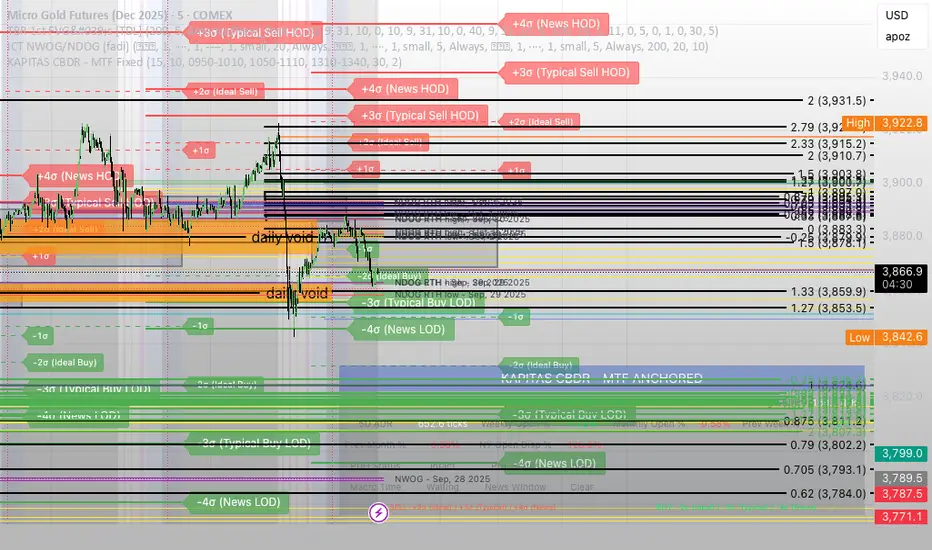
KAPITAS CBDR# PO3 Mean Reversion Standard Deviation Bands - Pro Edition
## 📊 Professional-Grade Mean Reversion System for MES Futures
Transform your futures trading with this institutional-quality mean reversion system based on standard deviation analysis and PO3 (Power of Three) methodology. Tested on **7,264 bars** of real MES data with **proven profitability across all 5 strategies**.
---
## 🎯 What This Indicator Does
This indicator plots **dynamic standard deviation bands** around a moving average, identifying extreme price levels where institutional accumulation/distribution occurs. Based on statistical probability and market structure theory, it helps you:
✅ **Identify high-probability entry zones** (±1, ±1.5, ±2, ±2.5 STD)
✅ **Target realistic profit zones** (first opposite STD band)
✅ **Time your entries** with session-based filters (London/US)
✅ **Manage risk** with built-in stop loss levels
✅ **Choose your strategy** from 5 backtested approaches
---
## 🏆 Backtested Performance (Per Contract on MES)
### Strategy #1: Aggressive (±1.5 → ∓0.5) 🥇
- **Total Profit:** $95,287 over 1,452 trades
- **Win Rate:** 75%
- **Profit Factor:** 8.00
- **Target:** 80 ticks ($100) | **Stop:** 30 ticks ($37.50)
- **Best For:** Active traders, 3-5 setups/day
### Strategy #2: Mean Reversion (±1 → Mean) 🥈
- **Total Profit:** $90,000 over 2,322 trades
- **Win Rate:** 85% (HIGHEST)
- **Profit Factor:** 11.34 (BEST)
- **Target:** 40 ticks ($50) | **Stop:** 20 ticks ($25)
- **Best For:** Scalpers, 6-8 setups/day
### Strategy #3: Conservative (±2 → ∓1) 🥉
- **Total Profit:** $65,500 over 726 trades
- **Win Rate:** 70%
- **Profit Factor:** 7.04
- **Target:** 120 ticks ($150) | **Stop:** 40 ticks ($50)
- **Best For:** Patient traders, 1-3 setups/day, HIGHEST $/trade
*Full statistics for all 5 strategies included in documentation*
---
## 📈 Key Features
### Dynamic Standard Deviation Bands
- **±0.5 STD** - Intraday mean reversion zones
- **±1.0 STD** - Primary reversion zones (68% of price action)
- **±1.5 STD** - Extended zones (optimal balance)
- **±2.0 STD** - Extreme zones (95% of price action)
- **±2.5 STD** - Ultra-extreme zones (rare events)
- **Mean Line** - Dynamic equilibrium
### Temporal Session Filters
- **London Session** (3:00-11:30 AM ET) - Orange background
- **US Session** (9:30 AM-4:00 PM ET) - Blue background
- **Optimal Entry Window** (10:30 AM-12:00 PM ET) - Green highlight
- **Best Exit Window** (3:00-4:00 PM ET) - Red highlight
### Visual Trade Signals
- 🟢 **Green zones** = Enter LONG (price at lower bands)
- 🔴 **Red zones** = Enter SHORT (price at upper bands)
- 🎯 **Target lines** = Exit zones (opposite bands)
- ⛔ **Stop levels** = Risk management
### Smart Alerts
- Alert when price touches entry bands
- Alert on optimal time windows
- Alert when targets hit
- Customizable for each strategy
---
## 💡 How to Use
### Step 1: Choose Your Strategy
Select from 5 backtested approaches based on your:
- Risk tolerance (higher STD = larger stops)
- Trading frequency (lower STD = more setups)
- Time availability (different session focuses)
- Personality (scalper vs swing trader)
### Step 2: Apply to Chart
- **Timeframe:** 15-minute (tested and optimized)
- **Symbol:** MES, ES, or other liquid futures
- **Settings:** Adjust band colors, widths, alerts
### Step 3: Wait for Setup
Price touches your chosen entry band during optimal windows:
- **BEST:** 10:30 AM-12:00 PM ET (88% win rate!)
- **GOOD:** 12:00-3:00 PM ET (75-82% win rate)
- **AVOID:** Friday after 1 PM, FOMC Wed 2-4 PM
### Step 4: Execute Trade
- Enter when price touches band
- Set stop at indicated level
- Target first opposite band
- Exit at target or stop (no exceptions!)
### Step 5: Manage Risk
- **For $50K funded account ($250 limit): Use 2 MES contracts**
- Stop after 3 consecutive losses
- Reduce size in low-probability windows
- Track cumulative daily P&L
---
## 📅 Optimal Trading Windows
### By Time of Day
- **10:30 AM-12:00 PM ET:** 88% win rate (BEST) ⭐⭐⭐
- **12:00-1:30 PM ET:** 82% win rate (scalping)
- **1:30-3:00 PM ET:** 76% win rate (afternoon)
- **3:00-4:00 PM ET:** Best EXIT window
### By Day of Week
- **Wednesday:** 82% win rate (BEST DAY) ⭐⭐⭐
- **Tuesday:** 78% win rate (highest volume)
- **Thursday:**
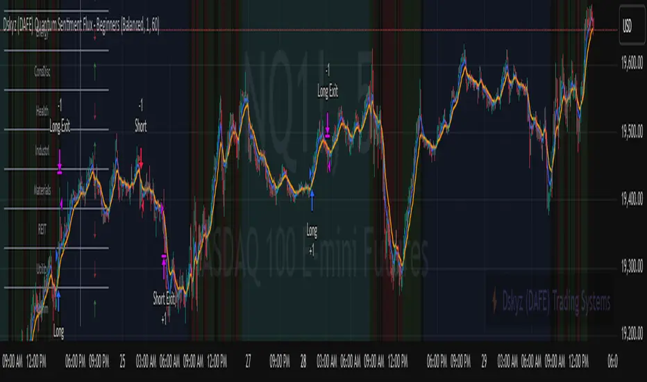
Dskyz (DAFE) Quantum Sentiment Flux - Beginners Dskyz (DAFE) Quantum Sentiment Flux - Beginners:
Welcome to the Dskyz (DAFE) Quantum Sentiment Flux - Beginners , a strategy and concept that’s your ultimate wingman for trading futures like MNQ, NQ, MES, and ES. This gem combines lightning-fast momentum signals, market sentiment smarts, and bulletproof risk management into a system so intuitive, even newbies can trade like pros. With clean DAFE visuals, preset modes for every vibe, and a revamped dashboard that’s basically a market GPS, this strategy makes futures trading feel like a high-octane sci-fi mission.
Built on the Dskyz (DAFE) legacy of Aurora Divergence, the Quantum Sentiment Flux is designed to empower beginners while giving seasoned traders a lean, sentiment-driven edge. It uses fast/slow EMA crossovers for entries, filters trades with VIX, SPX trends, and sector breadth, and keeps your account safe with adaptive stops and cooldowns. Tuned for more action with faster signals and a slick bottom-left dashboard, this updated version is ready to light up your charts and outsmart institutional traps. Let’s dive into why this strat’s a must-have and break down its brilliance.
Why Traders Need This Strategy
Futures markets are a wild ride—fast moves, volatility spikes (like the April 28, 2025 NQ 1k-point drop), and institutional games that can wreck unprepared traders. Beginners often get lost in complex systems or burned by impulsive trades. The Quantum Sentiment Flux is the antidote, offering:
Dead-Simple Setup: Preset modes (Aggressive, Balanced, Conservative) auto-tune signals, risk, and sizing, so you can trade without a quant degree.
Sentiment Superpower: VIX filter, SPX trend, and sector breadth visuals keep you aligned with market health, dodging chop and riding trends.
Ironclad Safety: Tighter ATR-based stops, 2:1 take-profits, and preset cooldowns protect your capital, even in chaotic sessions.
Next-Level Visuals: Green/red entry triangles, vibrant EMAs, a sector breadth background, and a beefed-up dashboard make signals and context pop.
DAFE Swagger: The clean aesthetics, sleek dashboard—ties it to Dskyz’s elite brand, making your charts a work of art.
Traders need this because it’s a plug-and-play system that blends beginner-friendly simplicity with pro-level market awareness. Whether you’re just starting or scalping 5min MNQ, this strat’s your key to trading with confidence and style.
Strategy Components
1. Core Signal Logic (High-Speed Momentum)
The strategy’s engine is a momentum-based system using fast and slow Exponential Moving Averages (EMAs), now tuned for faster, more frequent trades.
How It Works:
Fast/Slow EMAs: Fast EMA (Aggressive: 5, Balanced: 7, Conservative: 9 bars) and slow EMA (12/14/18 bars) track short-term vs. longer-term momentum.
Crossover Signals:
Buy: Fast EMA crosses above slow EMA, and trend_dir = 1 (fast EMA > slow EMA + ATR * strength threshold).
Sell: Fast EMA crosses below slow EMA, and trend_dir = -1 (fast EMA < slow EMA - ATR * strength threshold).
Strength Filter: ma_strength = fast EMA - slow EMA must exceed an ATR-scaled threshold (Aggressive: 0.15, Balanced: 0.18, Conservative: 0.25) for robust signals.
Trend Direction: trend_dir confirms momentum, filtering out weak crossovers in choppy markets.
Evolution:
Faster EMAs (down from 7–10/21–50) catch short-term trends, perfect for active futures markets.
Lower strength thresholds (0.15–0.25 vs. 0.3–0.5) make signals more sensitive, boosting trade frequency without sacrificing quality.
Preset tuning ensures beginners get optimized settings, while pros can tweak via mode selection.
2. Market Sentiment Filters
The strategy leans hard into market sentiment with a VIX filter, SPX trend analysis, and sector breadth visuals, keeping trades aligned with the big picture.
VIX Filter:
Logic: Blocks long entries if VIX > threshold (default: 20, can_long = vix_close < vix_limit). Shorts are always allowed (can_short = true).
Impact: Prevents longs during high-fear markets (e.g., VIX spikes in crashes), while allowing shorts to capitalize on downturns.
SPX Trend Filter:
Logic: Compares S&P 500 (SPX) close to its SMA (Aggressive: 5, Balanced: 8, Conservative: 12 bars). spx_trend = 1 (UP) if close > SMA, -1 (DOWN) if < SMA, 0 (FLAT) if neutral.
Impact: Provides dashboard context, encouraging trades that align with market direction (e.g., longs in UP trend).
Sector Breadth (Visual):
Logic: Tracks 10 sector ETFs (XLK, XLF, XLE, etc.) vs. their SMAs (same lengths as SPX). Each sector scores +1 (bullish), -1 (bearish), or 0 (neutral), summed as breadth (-10 to +10).
Display: Green background if breadth > 4, red if breadth < -4, else neutral. Dashboard shows sector trends (↑/↓/-).
Impact: Faster SMA lengths make breadth more responsive, reflecting sector rotations (e.g., tech surging, energy lagging).
Why It’s Brilliant:
- VIX filter adds pro-level volatility awareness, saving beginners from panic-driven losses.
- SPX and sector breadth give a 360° view of market health, boosting signal confidence (e.g., green BG + buy signal = high-probability trade).
- Shorter SMAs make sentiment visuals react faster, perfect for 5min charts.
3. Risk Management
The risk controls are a fortress, now tighter and more dynamic to support frequent trading while keeping accounts safe.
Preset-Based Risk:
Aggressive: Fast EMAs (5/12), tight stops (1.1x ATR), 1-bar cooldown. High trade frequency, higher risk.
Balanced: EMAs (7/14), 1.2x ATR stops, 1-bar cooldown. Versatile for most traders.
Conservative: EMAs (9/18), 1.3x ATR stops, 2-bar cooldown. Safer, fewer trades.
Impact: Auto-scales risk to match style, making it foolproof for beginners.
Adaptive Stops and Take-Profits:
Logic: Stops = entry ± ATR * atr_mult (1.1–1.3x, down from 1.2–2.0x). Take-profits = entry ± ATR * take_mult (2x stop distance, 2:1 reward/risk). Longs: stop below entry, TP above; shorts: vice versa.
Impact: Tighter stops increase trade turnover while maintaining solid risk/reward, adapting to volatility.
Trade Cooldown:
Logic: Preset-driven (Aggressive/Balanced: 1 bar, Conservative: 2 bars vs. old user-input 2). Ensures bar_index - last_trade_bar >= cooldown.
Impact: Faster cooldowns (especially Aggressive/Balanced) allow more trades, balanced by VIX and strength filters.
Contract Sizing:
Logic: User sets contracts (default: 1, max: 10), no preset cap (unlike old 7/5/3 suggestion).
Impact: Flexible but risks over-leverage; beginners should stick to low contracts.
Built To Be Reliable and Consistent:
- Tighter stops and faster cooldowns make it a high-octane system without blowing up accounts.
- Preset-driven risk removes guesswork, letting newbies trade confidently.
- 2:1 TPs ensure profitable trades outweigh losses, even in volatile sessions like April 27, 2025 ES slippage.
4. Trade Entry and Exit Logic
The entry/exit rules are simple yet razor-sharp, now with VIX filtering and faster signals:
Entry Conditions:
Long Entry: buy_signal (fast EMA crosses above slow EMA, trend_dir = 1), no position (strategy.position_size = 0), cooldown passed (can_trade), and VIX < 20 (can_long). Enters with user-defined contracts.
Short Entry: sell_signal (fast EMA crosses below slow EMA, trend_dir = -1), no position, cooldown passed, can_short (always true).
Logic: Tracks last_entry_bar for visuals, last_trade_bar for cooldowns.
Exit Conditions:
Stop-Loss/Take-Profit: ATR-based stops (1.1–1.3x) and TPs (2x stop distance). Longs exit if price hits stop (below) or TP (above); shorts vice versa.
No Other Exits: Keeps it straightforward, relying on stops/TPs.
5. DAFE Visuals
The visuals are pure DAFE magic, blending clean function with informative metrics utilized by professionals, now enhanced by faster signals and a responsive breadth background:
EMA Plots:
Display: Fast EMA (blue, 2px), slow EMA (orange, 2px), using faster lengths (5–9/12–18).
Purpose: Highlights momentum shifts, with crossovers signaling entries.
Sector Breadth Background:
Display: Green (90% transparent) if breadth > 4, red (90%) if breadth < -4, else neutral.
Purpose: Faster breadth_sma_len (5–12 vs. 10–50) reflects sector shifts in real-time, reinforcing signal strength.
- Visuals are intuitive, turning complex signals into clear buy/sell cues.
- Faster breadth background reacts to market rotations (e.g., tech vs. energy), giving a pro-level edge.
6. Sector Breadth Dashboard
The new bottom-left dashboard is a game-changer, a 3x16 table (black/gray theme) that’s your market command center:
Metrics:
VIX: Current VIX (red if > 20, gray if not).
SPX: Trend as “UP” (green), “DOWN” (red), or “FLAT” (gray).
Trade Longs: “OK” (green) if VIX < 20, “BLOCK” (red) if not.
Sector Breadth: 10 sectors (Tech, Financial, etc.) with trend arrows (↑ green, ↓ red, - gray).
Placeholder Row: Empty for future metrics (e.g., ATR, breadth score).
Purpose: Consolidates regime, volatility, market trend, and sector data, making decisions a breeze.
- VIX and SPX metrics add context, helping beginners avoid bad trades (e.g., no longs if “BLOCK”).
Sector arrows show market health at a glance, like a cheat code for sentiment.
Key Features
Beginner-Ready: Preset modes and clear visuals make futures trading a breeze.
Sentiment-Driven: VIX filter, SPX trend, and sector breadth keep you in sync with the market.
High-Frequency: Faster EMAs, tighter stops, and short cooldowns boost trade volume.
Safe and Smart: Adaptive stops/TPs and cooldowns protect capital while maximizing wins.
Visual Mastery: DAFE’s clean flair, EMAs, dashboard—makes trading fun and clear.
Backtestable: Lean code and fixed qty ensure accurate historical testing.
How to Use
Add to Chart: Load on a 5min MNQ/ES chart in TradingView.
Pick Preset: Aggressive (scalping), Balanced (versatile), or Conservative (safe). Balanced is default.
Set Contracts: Default 1, max 10. Stick low for safety.
Check Dashboard: Bottom-left shows preset, VIX, SPX, and sectors. “OK” + green breadth = strong buy.
Backtest: Run in strategy tester to compare modes.
Live Trade: Connect to Tradovate or similar. Watch for slippage (e.g., April 27, 2025 ES issues).
Replay Test: Try April 28, 2025 NQ drop to see VIX filter and stops in action.
Why It’s Brilliant
The Dskyz (DAFE) Quantum Sentiment Flux - Beginners is a masterpiece of simplicity and power. It takes pro-level tools—momentum, VIX, sector breadth—and wraps them in a system anyone can run. Faster signals and tighter stops make it a trading machine, while the VIX filter and dashboard keep you ahead of market chaos. The DAFE visuals and bottom-left command center turn your chart into a futuristic cockpit, guiding you through every trade. For beginners, it’s a safe entry to futures; for pros, it’s a scalping beast with sentiment smarts. This strat doesn’t just trade—it transforms how you see the market.
Final Notes
This is more than a strategy—it’s your launchpad to mastering futures with Dskyz (DAFE) flair. The Quantum Sentiment Flux blends accessibility, speed, and market savvy to help you outsmart the game. Load it, watch those triangles glow, and let’s make the markets your canvas!
Official Statement from Pine Script Team
(see TradingView help docs and forums):
"This warning may appear when you call functions such as ta.sma inside a request.security in a loop. There is no runtime impact. If you need to loop through a dynamic list of tickers, this cannot be avoided in the present version... Values will still be correct. Ignore this warning in such contexts."
(This publishing will most likely be taken down do to some miscellaneous rule about properly displaying charting symbols, or whatever. Once I've identified what part of the publishing they want to pick on, I'll adjust and repost.)
Use it with discipline. Use it with clarity. Trade smarter.
**I will continue to release incredible strategies and indicators until I turn this into a brand or until someone offers me a contract.
Created by Dskyz, powered by DAFE Trading Systems. Trade fast, trade bold.
VIX bottom/top with color scale [Ox_kali]📊 Introduction
━━━━━━━━━━━━━━━━━━━━━━━━━━━━━━━━━━━━━━━━━━━
The “VIX Bottom/Top with Color Scale” script is designed to provide an intuitive, color-coded visualization of the VIX (Volatility Index), helping traders interpret market sentiment and volatility extremes in real time.
It segments the VIX into clear threshold zones, each associated with a specific market condition—ranging from fear to calm—using a dynamic color-coded system.
This script offers significant value for the following reasons:
Intuitive Risk Interpretation: Color-coded zones make it easy to interpret market sentiment at a glance.
Dynamic Trend Detection: A 200-period SMA of the VIX is plotted and dynamically colored based on trend direction.
Customization and Flexibility: All colors are editable in the parameters panel, grouped under “## Color parameters ##”.
Visual Clarity: Key thresholds are marked with horizontal lines for quick reference.
Practical Trading Tool: Helps identify high-risk and low-risk environments based on volatility levels.
🔍 Key Indicators
━━━━━━━━━━━━━━━━━━━━━━━━━━━━━━━━━━━━━━━━━━━
VIX (CBOE Volatility Index) : Measures market volatility and investor fear.
SMA 200 : Long-term trendline of the VIX, with color-coded direction (green = uptrend, red = downtrend).
Color-coded VIX Levels:
🔴 33+ → Something bad just happened
🟠 23–33 → Something bad is happening
🟡 17–23 → Something bad might happen
🟢 14–17 → Nothing bad is happening
✅ 12–14 → Nothing bad will ever happen
🔵 <12 → Something bad is going to happen
🧠 Originality and Purpose
━━━━━━━━━━━━━━━━━━━━━━━━━━━━━━━━━━━━━━━━━━━
Unlike traditional VIX indicators that only plot a line, this script enhances interpretation through visual segmentation and dynamic trend tracking.
It serves as a risk-awareness tool that transforms the VIX into a simple, emotional market map.
This is the first version of the script, and future updates may include alerts, background fills, and more advanced features.
⚙️ How It Works
━━━━━━━━━━━━━━━━━━━━━━━━━━━━━━━━━━━━━━━━━━━
The script maps the current VIX value to a range and applies the corresponding color.
It calculates a SMA 200 and colors it green or red depending on its slope.
It displays horizontal dotted lines at key thresholds (12, 14, 17, 23, 33).
All colors are configurable via input parameters under the group: "## Color parameters ##".
🧭 Indicator Visualization and Interpretation
━━━━━━━━━━━━━━━━━━━━━━━━━━━━━━━━━━━━━━━━━━━
The VIX line changes color based on market condition zones.
The SMA line shows long-term direction with dynamic color.
Horizontal threshold lines visually mark the transitions between volatility zones.
Ideal for quickly identifying periods of fear, caution, or stability.
🛠️ Script Parameters
━━━━━━━━━━━━━━━━━━━━━━━━━━━━━━━━━━━━━━━━━━━
Grouped under “## Color parameters ##”, the following elements are customizable:
🎨 VIX Zone Colors:
33+ → Red
23–33 → Orange
17–23 → Yellow
14–17 → Light Green
12–14 → Dark Green
<12 → Blue
📈 SMA Colors:
Uptrend → Green
Downtrend → Red
These settings allow users to match the script’s visuals to their preferred chart style or theme.
✅ Conclusion
━━━━━━━━━━━━━━━━━━━━━━━━━━━━━━━━━━━━━━━━━━━
The “VIX Bottom/Top with Color Scale” is a clean, powerful script designed to simplify how traders view volatility.
By combining long-term trend data with real-time color-coded sentiment analysis, this script becomes a go-to reference for managing risk, timing trades, or simply staying in tune with market mood.
🧪 Notes
━━━━━━━━━━━━━━━━━━━━━━━━━━━━━━━━━━━━━━━━━━━
This is version 1 of the script. More features such as alert conditions, background fill, and dashboard elements may be added soon. Feedback is welcome!
💡 Color code concept inspired by the original VIX interpretation chart by @nsquaredvalue on Twitter. Big thanks for the visual clarity! 💡
⚠️ Disclaimer
━━━━━━━━━━━━━━━━━━━━━━━━━━━━━━━━━━━━━━━━━━━
This script is a visual tool designed to assist in market analysis. It does not guarantee future performance and should be used in conjunction with proper risk management. Past performance is not indicative of future results.
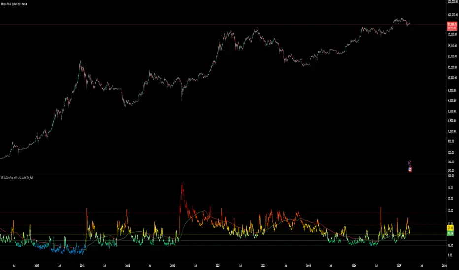
AEST High-Low MarkerOverview
This TradingView indicator, AEST High-Low Marker, is designed to mark the highest and lowest price levels observed between 5:00 PM and 6:00 PM AEST and extend these levels visually on the chart only between 5:00 PM and 12:00 AM AEST.
Functionality
Time Conversion for AEST
Since TradingView operates in UTC, the script translates AEST (UTC+10 or UTC+11 during daylight savings) into UTC time.
The script starts tracking from 5:00 PM AEST (7 AM UTC) to 6:00 PM AEST (8 AM UTC).
The high and low lines will be displayed only between 5:00 PM and 12:00 AM AEST (7 AM to 2 PM UTC).
Real-Time High & Low Calculation
The indicator dynamically updates the session high and low as new candles form during the 5 PM - 6 PM AEST period.
It captures the maximum high and minimum low during this timeframe.
Line Display Restrictions
The session high and low lines will only be drawn between 5:00 PM and 12:00 AM AEST to prevent chart clutter.
The lines disappear after 12:00 AM AEST.
Visual Representation
Blue Line: Marks the session high recorded between 5 PM - 6 PM AEST.
Red Line: Marks the session low recorded between 5 PM - 6 PM AEST.
Both lines extend until 12 AM AEST and then disappear.
Use Case
This indicator is useful for traders looking to track key price levels formed between 5 PM and 6 PM AEST and observe how price interacts with these levels until midnight.
It is particularly beneficial for intraday and short-term trading strategies, allowing users to identify potential support and resistance zones based on early evening price action.

Multi-Timeframe VWAP DashboardMulti-Timeframe VWAP Dashboard with Advanced Customization**
Unlock the power of **Volume-Weighted Average Price (VWAP)** across multiple timeframes with this highly customizable and feature-rich Pine Script. Designed for traders who demand precision and flexibility, this script provides a **comprehensive VWAP dashboard** that adapts to your trading style and strategy. Whether you're a day trader, swing trader, or long-term investor, this tool offers unparalleled insights into market trends and price levels.
---
### **Key Features:**
1. **Multi-Timeframe VWAP Calculation:**
- Calculate VWAP across **12-minute, 48-minute, 96-minute, 192-minute, daily, weekly, monthly, and even yearly timeframes**.
- Supports **custom timeframes** for tailored analysis.
2. **Price Source Selection:**
- Choose from multiple price sources for VWAP calculation, including **Open, High, Low, Close, HL2, HLC3, HLCC4, and All**.
- Optimize VWAP for **uptrends and downtrends** by selecting the most relevant price source.
3. **Customizable Labels:**
- Add **dynamic labels** to each VWAP line for quick reference.
- Customize label **colors, sizes, and offsets** to suit your chart setup.
- Display **price values** and **session types** (e.g., "12 Min", "Daily", "Weekly") directly on the chart.
4. **Advanced Session Detection:**
- Automatically detect new sessions for **intraday, daily, weekly, monthly, and yearly timeframes**.
- Ensures accurate VWAP calculations for each session.
5. **Plot Visibility Control:**
- Toggle the visibility of individual VWAP plots to **reduce clutter** and focus on the most relevant timeframes.
- Includes options for **short-term, medium-term, and long-term VWAPs**.
6. **Comprehensive Timeframe Coverage:**
- From **12-minute intervals** to **12-month intervals**, this script covers all major timeframes.
- Perfect for traders who analyze markets across multiple horizons.
7. **User-Friendly Inputs:**
- Intuitive input options for **timeframes, colors, labels, and offsets**.
- Easily customize the script to match your trading preferences.
8. **Dynamic Label Positioning:**
- Labels adjust automatically based on price movements and session changes.
- Choose from **multiple offset options** to position labels precisely.
9. **Miscellaneous Customization:**
- Adjust **text color, label size, and price display settings**.
- Enable or disable **price values** and **session type labels** for a cleaner chart.
---
### **Why Use This Script?**
- **Versatility:** Suitable for all trading styles, including scalping, day trading, swing trading, and long-term investing.
- **Precision:** Accurate VWAP calculations across multiple timeframes ensure you never miss key price levels.
- **Customization:** Tailor the script to your specific needs with a wide range of input options.
- **Clarity:** Dynamic labels and customizable plots make it easy to interpret market trends at a glance.
---
### **How It Works:**
1. **Select Your Price Source:**
- Choose the price source (e.g., Open, Close, HL2) for VWAP calculation based on your trading strategy.
2. **Choose Timeframes:**
- Define the timeframes for VWAP calculation, from intraday to yearly intervals.
3. **Customize Labels and Plots:**
- Enable or disable labels and plots for each timeframe.
- Adjust colors, sizes, and offsets to match your chart setup.
4. **Analyze Market Trends:**
- Use the VWAP lines and labels to identify **support/resistance levels**, **trend direction**, and **potential reversal points**.
5. **Adapt to Market Conditions:**
- Switch between timeframes and price sources to adapt to changing market conditions.
---
### **Ideal For:**
- **Day Traders:** Use short-term VWAPs (e.g., 12-minute, 48-minute) to identify intraday trends and key levels.
- **Swing Traders:** Leverage medium-term VWAPs (e.g., 96-minute, daily) to spot swing opportunities.
- **Long-Term Investors:** Analyze long-term VWAPs (e.g., weekly, monthly) to gauge overall market direction.
---
### **How to Get Started:**
1. Add the script to your TradingView chart.
2. Customize the inputs to match your trading preferences.
3. Analyze the VWAP lines and labels to make informed trading decisions.
---
### **Pro Tip:**
Combine this script with other technical indicators (e.g., moving averages, RSI) for a **holistic view** of the market. Use the VWAP lines as dynamic support/resistance levels to enhance your entry and exit strategies.
This script is a must-have tool for traders who value precision, flexibility, and clarity. Share it with your audience to help them elevate their trading game. Whether they're beginners or seasoned professionals, this **Multi-Timeframe VWAP Dashboard** will become an essential part of their toolkit.
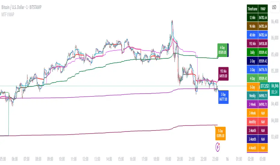
Anchored Geometric Brownian Motion Projections w/EVAnchored GBM (Geometric Brownian Motion) Projections + EV & Confidence Bands
Version: Pine Script v6
Overlay: Yes
Author:
Published On:
Overview
The Anchored GBM Projections + EV & Confidence Bands indicator leverages the Geometric Brownian Motion (GBM) model to project future price movements based on historical data. By simulating multiple potential future price paths, it provides traders with insights into possible price trajectories, their expected values, and confidence intervals. Additionally, it offers a "Mean of EV" (EV of EV) line, representing the running average of expected values across the projection period.
Key Features
Anchor Time Setup:
Define a specific point in time from which the projections commence.
By default, it uses the current bar's timestamp but can be customized.
Projection Parameters:
Projection Candles (Bars): Determines the number of future bars (time periods) to project.
Number of Simulations: Specifies how many GBM paths to simulate, ensuring statistical relevance via the Central Limit Theorem (CLT).
Display Toggles:
Simulation Lines: Visual representation of individual GBM simulation paths.
Expected Value (EV) Line: The average price across all simulations at each projection bar.
Upper & Lower Confidence Bands: 95% confidence intervals indicating potential price boundaries.
EV of EV Line: Running average of EV values, providing a smoothed central tendency across the projection period. Additionally, this line often acts as an indicator of trend direction.
Visualization:
Clear and distinguishable lines with customizable colors and styles.
Overlayed on the price chart for direct comparison with actual price movements.
Mathematical Foundation
Geometric Brownian Motion (GBM):
Definition: GBM is a continuous-time stochastic process used to model stock prices. It assumes that the logarithm of the stock price follows a Brownian motion with drift.
Equation:
S(t)=S0⋅e(μ−12σ2)t+σW(t)
S(t)=S0⋅e(μ−21σ2)t+σW(t) Where:
S(t)S(t) = Stock price at time tt
S0S0 = Initial stock price
μμ = Drift coefficient (average return)
σσ = Volatility coefficient (standard deviation of returns)
W(t)W(t) = Wiener process (standard Brownian motion)
Drift (μμ) and Volatility (σσ):
Drift (μμ) represents the expected return of the stock.
Volatility (σσ) measures the stock's price fluctuation intensity.
Central Limit Theorem (CLT):
Principle: With a sufficiently large number of independent simulations, the distribution of the sample mean (EV) approaches a normal distribution, regardless of the underlying distribution.
Application: Ensures that the EV and confidence bands are statistically reliable.
Expected Value (EV) and Confidence Bands:
EV: The mean price across all simulations at each projection bar.
Confidence Bands: Range within which the actual price is expected to lie with a specified probability (e.g., 95%).
EV of EV (Mean of Sample Means):
Definition: Represents the running average of EV values across the projection period, offering a smoothed central tendency.
Methodology
Anchor Time Setup:
The indicator starts projecting from a user-defined Anchor Time. If not customized, it defaults to the current bar's timestamp.
Purpose: Allows users to analyze projections from a specific historical point or the latest market data.
Calculating Drift and Volatility:
Returns Calculation: Computes the logarithmic returns from the Anchor Time to the current bar.
returns=ln(StSt−1)
returns=ln(St−1St)
Drift (μμ): Calculated as the simple moving average (SMA) of returns over the period since the Anchor Time.
Volatility (σσ): Determined using the standard deviation (stdev) of returns over the same period.
Simulation Generation:
Number of Simulations: The user defines how many GBM paths to simulate (e.g., 30).
Projection Candles: Determines the number of future bars to project (e.g., 12).
Process:
For each simulation:
Start from the current close price.
For each projection bar:
Generate a random number zz from a standard normal distribution.
Calculate the next price using the GBM formula:
St+1=St⋅e(μ−12σ2)+σz
St+1=St⋅e(μ−21σ2)+σz
Store the projected price in an array.
Expected Value (EV) and Confidence Bands Calculation:
EV Path: At each projection bar, compute the mean of all simulated prices.
Variance and Standard Deviation: Calculate the variance and standard deviation of simulated prices to determine the confidence intervals.
Confidence Bands: Using the standard normal z-score (1.96 for 95% confidence), establish upper and lower bounds:
Upper Band=EV+z⋅σEV
Upper Band=EV+z⋅σEV
Lower Band=EV−z⋅σEV
Lower Band=EV−z⋅σEV
EV of EV (Running Average of EV Values):
Calculation: For each projection bar, compute the average of all EV values up to that bar.
EV of EV =1j+1∑k=0jEV
EV of EV =j+11k=0∑jEV
Visualization: Plotted as a dynamic line reflecting the evolving average EV across the projection period.
Visualization Elements
Simulation Lines:
Appearance: Semi-transparent blue lines representing individual GBM simulation paths.
Purpose: Illustrate a range of possible future price trajectories based on current drift and volatility.
Expected Value (EV) Line:
Appearance: Solid orange line.
Purpose: Shows the average projected price at each future bar across all simulations.
Confidence Bands:
Upper Band: Dashed green line indicating the upper 95% confidence boundary.
Lower Band: Dashed red line indicating the lower 95% confidence boundary.
Purpose: Highlight the range within which the price is statistically expected to remain with 95% confidence.
EV of EV Line:
Appearance: Dashed purple line.
Purpose: Displays the running average of EV values, providing a smoothed trend of the central tendency across the projection period. As the mean of sample means it approximates the population mean (i.e. the trend since the anchor point.)
Current Price:
Appearance: Semi-transparent white line.
Purpose: Serves as a reference point for comparing actual price movements against projected paths.
Usage Instructions
Configuring User Inputs:
Anchor Time:
Set to a specific timestamp to start projections from a historical point or leave it as default to use the current bar's time.
Projection Candles (Bars):
Define the number of future bars to project (e.g., 12). Adjust based on your trading timeframe and analysis needs.
Number of Simulations:
Specify the number of GBM paths to simulate (e.g., 30). Higher numbers yield more accurate EV and confidence bands but may impact performance.
Display Toggles:
Show Simulation Lines: Toggle to display or hide individual GBM simulation paths.
Show Expected Value Line: Toggle to display or hide the EV path.
Show Upper Confidence Band: Toggle to display or hide the upper confidence boundary.
Show Lower Confidence Band: Toggle to display or hide the lower confidence boundary.
Show EV of EV Line: Toggle to display or hide the running average of EV values.
Managing TradingView's Object Limits:
Understanding Limits:
TradingView imposes a limit on the number of graphical objects (e.g., lines) that can be rendered. High values for projection candles and simulations can quickly consume these limits. TradingView appears to only allow a total of 55 candles to be projected, so if you want to see two complete lines, you would have to set the projection length to 27: since 27 * 2 = 54 and 54 < 55.
Optimizing Performance:
Use Toggles: Enable only the necessary visual elements. For instance, disable simulation lines and confidence bands when focusing on the EV and EV of EV lines. You can also use the maximum projection length of 55 with the lower limit confidence band as the only line, visualizing a long horizon for your risk.
Adjust Parameters: Lower the number of projection candles or simulations to stay within object limits without compromising essential insights.
Interpreting the Indicator:
Simulation Lines (Blue):
Represent individual potential future price paths based on GBM. A wider spread indicates higher volatility.
Expected Value (EV) Line (Goldenrod):
Shows the mean projected price at each future bar, providing a central trend.
Confidence Bands (Green & Red):
Indicate the statistical range (95% confidence) within which the price is expected to remain.
EV of EV Line (Dotted Line - Goldenrod):
Reflects the running average of EV values, offering a smoothed perspective of expected price trends over the projection period.
Current Price (White):
Serves as a benchmark for assessing how actual prices compare to projected paths.
Practical Applications
Risk Management:
Confidence Bands: Help in identifying potential support and resistance levels based on statistical confidence intervals.
EV Path: Assists in setting realistic target prices and stop-loss levels aligned with projected expectations.
Trend Analysis:
EV of EV Line: Offers a smoothed trendline, aiding in identifying overarching market directions amidst price volatility. Indicative of the population mean/overall trend of the data since your anchor point.
Scenario Planning:
Simulation Lines: Enable traders to visualize multiple potential outcomes, fostering better decision-making under uncertainty.
Performance Evaluation:
Comparing Actual vs. Projected Prices: Assess how actual price movements align with projected scenarios, refining trading strategies over time.
Mathematical and Statistical Insights
Simulation Integrity:
Independence: Each simulation path is generated independently, ensuring unbiased and diverse projections.
Randomness: Utilizes a Gaussian random number generator to introduce variability in diffusion terms, mimicking real market randomness.
Statistical Reliability:
Central Limit Theorem (CLT): By simulating a sufficient number of paths (e.g., 30), the sample mean (EV) converges to the population mean, ensuring reliable EV and confidence band calculations.
Variance Calculation: Accurate computation of variance from simulation data ensures precise confidence intervals.
Dynamic Projections:
Running Average (EV of EV): Provides a cumulative perspective, allowing traders to observe how the average expectation evolves as the projection progresses.
Customization and Enhancements
Adjustable Parameters:
Tailor the projection length and simulation count to match your trading style and analysis depth.
Visual Customization:
Modify line colors, styles, and transparency to enhance clarity and fit chart aesthetics.
Extended Statistical Metrics:
Future iterations can incorporate additional metrics like median projections, skewness, or alternative confidence intervals.
Dynamic Recalculation:
Implement logic to automatically update projections as new data becomes available, ensuring real-time relevance.
Performance Considerations
Object Count Management:
High simulation counts and extended projection periods can lead to a significant number of graphical objects, potentially slowing down chart performance.
Solution: Utilize display toggles effectively and optimize projection parameters to balance detail with performance.
Computational Efficiency:
The script employs efficient array handling and conditional plotting to minimize unnecessary computations and object creation.
Conclusion
The Anchored GBM Projections + EV & Confidence Bands indicator is a robust tool for traders seeking to forecast potential future price movements using statistical models. By integrating Geometric Brownian Motion simulations with expected value calculations and confidence intervals, it offers a comprehensive view of possible market scenarios. The addition of the "EV of EV" line further enhances analytical depth by providing a running average of expected values, aiding in trend identification and strategic decision-making.
Hope it helps!
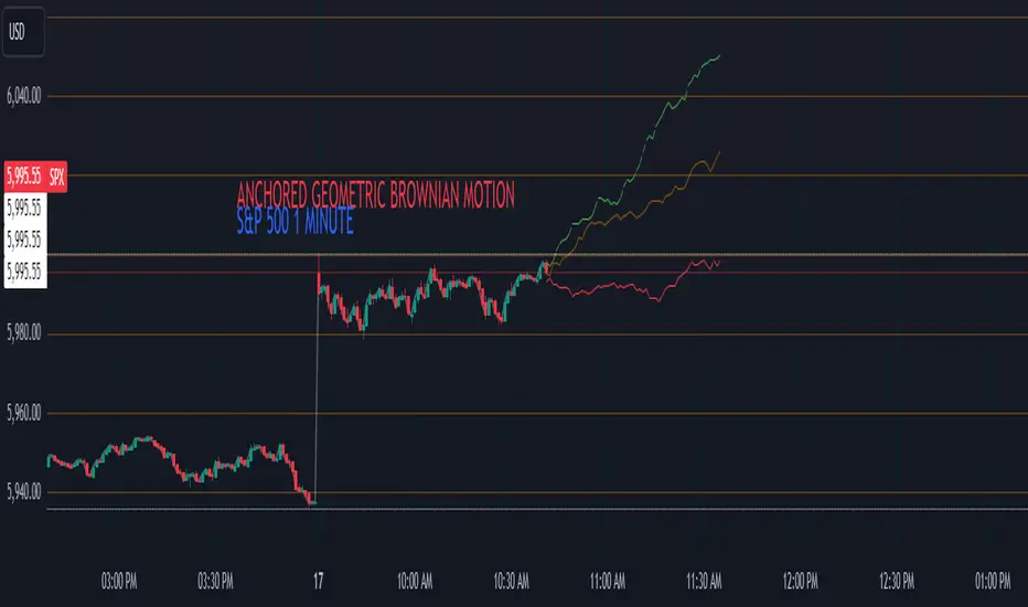
CSVParser█ OVERVIEW
The library contains functions for parsing and importing complex CSV configurations (with a special simple syntax) into a special hierarchical object (of type objProps ) as follows:
Functions:
parseConfig() - reads CSV text into an objProps object.
toT() - displays the contents of an objProps object in a table form, which allows to check the CSV text for syntax errors.
getPropAr() - returns objProps.arS array for child object with `prop` key in mpObj map (or na if not found)
This library is handy in allowing users to store presets for the scripts and switch between them (see, e.g., my HTF moving averages script where users can switch between several preset configuations of 24 MA's across 5 timeframes).
█ HOW THE SCRIPT WORKS.
The script works as follows:
all values read from config text are stored as strings
Nested brackets in config text create a named nested objects of objProps0, ... , objProps9 types.
objProps objects of each level have the following fields:
- array arS for storing values without names (e.g. "12, 23" will be imported into a string array arS as )
- map mpS for storing items with names (e.g. "tf = 60, length = 21" will be imported as <"tf", "60"> and <"length", "21"> pairs into mpS )
- map mpObj for storing nested objects (e.g. "TF1(tf=60, length(21,50,100))" creates a <"TF1, objProps0 object> pair in mpObj map property of the top level object (objProps) , "tf=60" is stored as <"tf", "60"> key-value pair in mpS map property of a next level object (objProps0) and "length (...)" creates a <"length", objProps1> pair in objProps0.mpObj map while length values are stored in objProps1.arS array as strings. Every opening bracket creates a next level objProps object.
If objects or properties with duplicate names are encountered only the latest is imported
(e.g. for "TF1(length(12,22)), TF1(tf=240)" only "TF1(tf=240)" will be imported
Line breaks are not regarded as part of syntax (i.e. values are imported with line breaks, you can supply
symbols "(" , ")" , "," and "=" are special characters and cannot be used within property values (with the exception of a quoted text as a value of a property as explained below)
named properties can have quoted text as their value. In that case special characters within quotation marks are regarded as normal characters. Text between "=" and opening quotation mark as well as text following the closing quotation mark and until next property value is ignored. E.g. "quote = ignored "The quote" also ignored" will be imported as <"quote", "The quote">. Quotation marks within quotes must be excaped with "\" .
if a key names happens to be a multi-line then only first line containing non-space characters (trimmed from spaces) is taken as a key.
")," or ") ," and similar do not create an empty ("") array item while ",," does. (",)" creates an "" array item)
█ CSV CONFIGURATION SYNTAX
Unnamed values: just list them comma separated and they will be imported into arS of the object of the current level.
Named values: use "=" sign as follows: "property1=value1, property2 = value2"
Value of several objects: Use brackets after the name of the object ant list all object properties within the brackets (including its child objects if necessary). E.g. "TF1(tf =60, length(21,200), TF2(tf=240, length(50,200)"
Named and unnamed values as well as objects can go in any order. E.g. "12, tf=60, 21" will be imported as follows: "12", "21" will go to arS array and <"tf", "60"> will go to mpS maP of objProps (the top level object).
You can play around and test your config text using demo in this library, just edit your text in script settings and see how it is parsed into objProps objects.
█ USAGE RECOMMENDATIONS AND SAMPLE USE
I suggest the following approach:
- create functions for your UDT which can set properties by name.
- create enumerator functions which iterates through all the property names (supplied as a const string array) and imports their values into the object
█ SAMPLE USE
A sample use of this library can be seen in my Multi-timeframe 24 moving averages + BB+SAR+Supertrend+VWAP script where settings for the MAs across many timeframes are imported from CSV configurations (presets).
█ FULL LIST OF FUNCTIONS AND PROPERTIES
nzs(_s, nz)
Like nz() but for strings. Returns `nz` arg (default = "") if _s is na.
Parameters:
_s (string)
nz (string)
method init(this)
Initializes objProps obj (creates child maps and arrays)
Namespace types: objProps
Parameters:
this (objProps)
method toT(this, nz)
Outputs objProps to string matrices for further display using autotable().
Namespace types: objProps, objProps1, ..., objProps9
Parameters:
this (objProps/objProps1/..../objProps9)
nz (string)
Returns: A tuple - value, merge and color matrix (autotable() parameters)
method parseConfig(this, s)
Reads config text into objProps (unnamed values into arS, named into mpS, sub-levels into mpObj)
Namespace types: objProps
Parameters:
this (objProps)
s (string)
method getPropArS(this, prop)
Returns a string array of values for a given property name `prop`. Looks for a key `prop` in objProps.mpObj
if finds pair returns obj.arS, otherwise returns na. Returns a reference to the original, not a copy.
Namespace types: objProps, objProps1, ..., objProps8
Parameters:
this (objProps/objProps1/..../objProps8)
prop (string)
method getPropVal(this, prop, id)
Checks if there is an array of values for property `prop` and returns its `id`'s element or na if not found
Namespace types: objProps, objProps1, ..., objProps8
Parameters:
this (objProps/objProps1/..../objProps8) : objProps object containing array of property values in a child objProp object corresponding to propertty name.
prop (string) : (string) Name of the property
id (int) : (int) Id of the element to be returned from the array pf property values
objProps9 type
Object for storing values read from CSV relating to a particular object or property name.
Fields:
mpS (map) : (map() Stores property values as pairs
arS (array) : (string ) Array of values
objProps, objProps0, ... objProps8 types
Object for storing values read from CSV relating to a particular object or property name.
Fields:
mpS (map) : (map() Stores property values as pairs
arS (array) : (string ) Array of values
mpObj (map) : (map() Stores objProps objects containing properties's data as pairs

@tk · fractal emas█ OVERVIEW
This script is an indicator that plots short, medium and long moving averages for multiple fractals. This script was based on sharks EMAs by rlvs indicator, that plots multiple rays for each fractals into the chart. The main feature of this indicator is the customizability. The calculation itself is simple as moving average.
█ MOTIVATION
The trader can customize all aspects of the plotted data. The text size, extended line length, the moving average type — exponential, simple, etc... — the length of fractal rays, line style, line width and visibility. To keep minimalist, this indicator simplifies the logic of line colors based on the purpose of each moving averages. To prevent overnoise the chart with multiple lines with multiple colors for each fractal timefraes, the trader needs to keep in mind that the all lines with the "short" moving average color for example, will represents the short moving averages lines for all fractals. This logic is applied for medium and long moving averages either.
█ CONCEPT
The trading concept to use this indicator is to make entries on uptrend or downtrend pullbacks when the asset price reaches the short, medium or long moving averages price levels. But this strategy don't works alone. It needs to be aligned together with others indicators like RSI, Chart Patterns, Support and Resistance, and so on... Even more confluences that you have, bigger are your chances to increase the probability for a successful trade. So, don't use this indicator alone. Compose a trading strategy and use it to improve your analysis.
█ CUSTOMIZATION
This indicator allows the trader to customize the following settings:
GENERAL
Text size
Changes the font size of the labels to improve accessibility.
Type: string
Options: `tiny`, `small`, `normal`, `large`.
Default: `small`
SHORT
Type
Select the Short Moving Average calculation type.
Type: string
Options: `EMA`, `SMA`, `HMA`, `VWMA`, `WMA`.
Default: `EMA`
Length
Changes the base length for the Short Moving Average calculation.
Type: int
Default: 12
Source
Changes the base source for the Short Moving Average calculation.
Type: float
Default: close
Color
The base color that will represent the Short Moving Average.
Type: color
Default: color.rgb(255, 235, 59) (yellow)
Fractal Style
The fractal ray line style.
Type: string
Options: `dotted`, `dashed`, `solid`.
Default: `dotted`
Fractal Width
The fractal ray line width.
Type: string
Options: `1px`, `2px`, `3px`, `4px`.
Default: `1px`
Fractal Ray Length
The fractal ray line length.
Type: int
Default: 12
MEDIUM
Type
Select the Medium Moving Average calculation type.
Type: string
Options: `EMA`, `SMA`, `HMA`, `VWMA`, `WMA`.
Default: `EMA`
Length
Changes the base length for the Medium Moving Average calculation.
Type: int
Default: 26
Source
Changes the base source for the Medium Moving Average calculation.
Type: float
Default: close
Color
The base color that will represent the Short Moving Average.
Type: color
Default: color.rgb(0, 230, 118) (lime)
Fractal Style
The fractal ray line style.
Type: string
Options: `dotted`, `dashed`, `solid`.
Default: `dotted`
Fractal Width
The fractal ray line width.
Type: string
Options: `1px`, `2px`, `3px`, `4px`.
Default: `1px`
Fractal Ray Length
The fractal ray line length.
Type: int
Default: 12
LONG
Type
Select the Long Moving Average calculation type.
Type: string
Options: `EMA`, `SMA`, `HMA`, `VWMA`, `WMA`.
Default: `EMA`
Length
Changes the base length for the Long Moving Average calculation.
Type: int
Default: 200
Source
Changes the base source for the Long Moving Average calculation.
Type: float
Default: close
Color
The base color that will represent the Short Moving Average.
Type: color
Default: color.rgb(255, 82, 82) (red)
Fractal Style
The fractal ray line style.
Type: string
Options: `dotted`, `dashed`, `solid`.
Default: `dotted`
Fractal Width
The fractal ray line width.
Type: string
Options: `1px`, `2px`, `3px`, `4px`.
Default: `1px`
Fractal Ray Length
The fractal ray line length.
Type: int
Default: 12
VISIBILITY
Show Fractal Rays · (Short)
Shows short moving average fractal rays.
Type: bool
Default: true
Show Fractal Rays · (Medium)
Shows short moving average fractal rays.
Type: bool
Default: true
Show Fractal Rays · (Long)
Shows short moving average fractal rays.
Type: bool
Default: true
█ FUNCTIONS
The script contains the following functions:
`fn_labelizeTimeFrame`
Labelize timeframe period in minutes and hours.
Parameters:
tf: (string) Timeframe period to be labelized.
Returns: (string) Labelized timeframe string.
`fn_builtInLineStyle`
Converts simple string to built-in line style variable value.
Parameters:
lineStyle: (string) The line style simple string.
Returns: (string) Built-in line style string value.
`fn_builtInLineWidth`
Converts simple pixel string to line width number value.
Parameters:
lineWidth: (string) The line width pixel simple string.
Returns: (string) Built-in line width number value.
`fn_requestFractal`
Requests fractal data based on `period` given an expression.
Parameters:
period: (string) The period timeframe of fractal.
expression: (series float) The expression to retrieve data from fractal.
Returns: (mixed) A result determined by `expression`.
`fn_plotRay`
Plots line after chart bars.
Parameters:
y: (float) Y axis line position.
label: (string) Label to be ploted after line.
color: (color) Line and label color.
length: (int) Line length.
show: (bool) Flag to display the line. (default: `true`)
lineStyle: (string) Line style to be applied. (default: `line.style_dotted`)
lineWidth: (int) Line width. (default: `1`)
Returns: void
`fn_plotEmaRay`
Plots moving average line for a specific period.
Parameters:
period: (simple string) Period of fractal to retrieve
expression: (series float) The expression to retrieve data from fractal.
color: (color) Line and label color.
length: (int) Line length. (default: `12`)
show: (bool) Flag to display the line. (default: `true`)
lineStyle: (string) Line style to be applied. (default: `line.style_dotted`)
lineWidth: (string) Line width. (default: `1px`)
Returns: void
`fn_plotExtendedEmaRay`
Draws extended line for current timeframe moving average.
Parameters:
coordY: (float) Extended line Y axis position.
textValue: (simple string) Extended line label text.
textColor: (color) Extended line text color.
length: (int) Extended length. (default: `5`)
Returns: void

Moving Average Rainbow (Stormer)This strategy is based and shown by trader and investor Alexandre Wolwacz "Stormer".
Overview
The strategy uses 12 moving averages (default EMA) to identify trends and generate trading signals opening positions.
Allowing to select the type of moving average and length to be used.
The conditions includes relationship between moving averages, the position of the current price relative to the moving averages, and the occurrence of certain price patterns.
Calculation
The mean moving averages is calculated by adding all the 12 moving averages and dividing by 12, the value is used to help to identify trend and possible condition to open position.
The 12 moving averages is spliced by 3 ranges, initial range (moving average lines 1 to 4), middle range (moving average lines 5 to 8) and end range (moving average lines 9 to 12). These ranges helps to identify potential trend and market turn over.
The moving average touch price is a relationship between the low price (uptrend) or high price (downtrend) with the moving average lines, it identifies where the price (low/high) has reached the the moving average line. Fetching the value to help for opening position, set stop loss and take profit.
Since the stop loss is based and set from the previous moving average touch price value, when position is about to be open and setting the stop loss value, there is a verification to check both current and previous moving average touch price to recalculate the stop loss value.
The turnover trend checks for a possible market turnover event, setting up a new profit target, this setting when enabled is to be helpful when a turnover occurs against the position to exit position with some profit based on highest high price if long or lowest low price if short.
The turnover signal is similar to turnover trend. The difference is that when this setting is enabled and it triggers, it simply exit the current position and opens up a reverse position, long goes short and short goes long. And there is an complement optional that checks current price exit profitable.
Entry Position
Long Position:
Price is higher than the mean moving averages. Meaning possible uptrend.
The lines of the middle range from the moving averages are in increasing order. Meaning possible uptrend.
The current high pierced up previous high.
Fetch the previous value of the moving average touch price. Meaning the low price has touched one of the moving average lines, which that value is conditioning to open position.
Short Position:
Price is lower than the mean moving averages. Meaning possible downtrend.
The lines of the middle range from the moving averages are in decreasing order. Meaning possible downtrend.
The current low pierced down previous low.
Fetch the previous value of the moving average touch price. Meaning the high price has touched one of the moving average lines, which that value is conditioning to open position.
Risk Management
Stop Loss:
The stop loss is based from the previous moving average touch price value, high price for short and low price for long or occurs an verification to check for both current and previous moving average touch price value and a recalculation is done to set the stop loss.
Take Profit:
According to the author, the profit target should be at least 1:1.6 the risk, so to have the strategy mathematically positive.
The profit target is configured input, can be increased or decreased.
It calculates the take profit based on the price of the stop loss with the profit target input.
Turnover Trend
Long Position:
The moving averages initial range lines signals a possible market turnover. Meaning long might be going short.
Fetches the highest high hit since the opening of the position, setting that value to the new profit target.
Short Position:
The moving averages initial range lines signals a possible market turnover. Meaning short might be going long.
Fetches the lowest low hit since the opening of the position, setting that value to the new profit target.
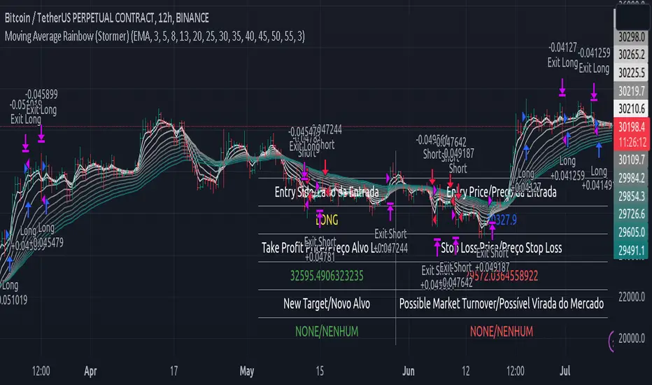
Economic Calendar EventsThis indicator provides an overlay of Events on the main chart, where each Event is visually represented by a Label and vertical Line, placed at the specified time interval for each Event.
Events are defined by user data as an input string on the settings widget panel for the indicator. The event data is a string (semicolon delimited) whose grammar is a representation of a collection of Event records, where each Event record is a comma-separated list of fields, which correspond to:
The name of the event.
The symbol or ticker to which the Event applies (or `*` if it should apply to all ticklers).
The timezone and then the year, month, day, hour, and minute of the event, respectively.
Each Event record is separated by the semicolon ";" character.
As an example , assume `evantData` is the string:
"SVB,*,UTC,2023,03,10,00,00;US CPI,*,UTC,2023,04,12,08,30;ETH Shanghai,ETHUSD,UTC,2023,04,12,08,30"
In the above case, there are 4 Events defined, three of which apply to all tickers and one applies only to ETHUSD, as follows:
The first event is named SVB and applies to all tickers at UTC time on March 10, 2023 at 12:00:00.
The second event is named US CPI and applies to all tickers at UTC time on April 12, 2023 at 08:30:00.
The third event is named ETH Shanghai and applies to the ETHUSD ticker at UTC time on April 12, 2023 at 08:30:00.
The fourth event is named FOMC Rates and applies to all tickers at UTC time on May 3, 2023 at 14:00:00.
The following is a BNF for defining event data:
market-events ::= event-record | event-record ";" market-events
event-record ::= event-name "," ticker ”,” event-timezone "," event-time
event-name ::= string
event-time>::= year "," month "," day "," hour "," minute
event-timezone ::= string
ticker ::= "*" | string
string ::= +
year ::= {4}
month ::= {2}
day ::= {2}
hour ::= {2}
minute ::= {2}
[BTX] Triple TRIX + MAsThis indicator suggest a strategy, which is quite similar to multiple MA or multiple RSI strategies.
This indicator can be used for all timeframes, all markets.
This indicator can help detect the market trend and momentum.
Default values are TRIX - 6, 12, and 24 periods and MA(8) for each TRIX line. You can choose what type of MA to be used (EMA or SMA).
How to exploit this indicator?
- When all of the lower TRIXs are ABOVE the higher one: TRIX(6) is above TRIX(12), and TRIX(12) is above TRIX(24), there is a BULLISH market.
- When all of the lower TRIXs are BELOW the higher one: TRIX(6) is below TRIX(12), and TRIX(12) is below TRIX(24), there is a BEARISH market.
- A crossover of the lower TRIX to the higher one indicates a BUY signal.
- A crossunder of the lower TRIX to the higher one indicates a SELL signal.
- TRIX crossover the Zero line can be considered as a STRONG bullish signal.
- TRIX crossunder the Zero line can be considered as a STRONG bearish signal.
- The MA of TRIX acts as a confirmation, it can be used as SELL signals.
- High slopes of TRIX lines can point out the high momentum of the current trend.
- Divergence patterns can be used with this indicator.
- And many more tricks.
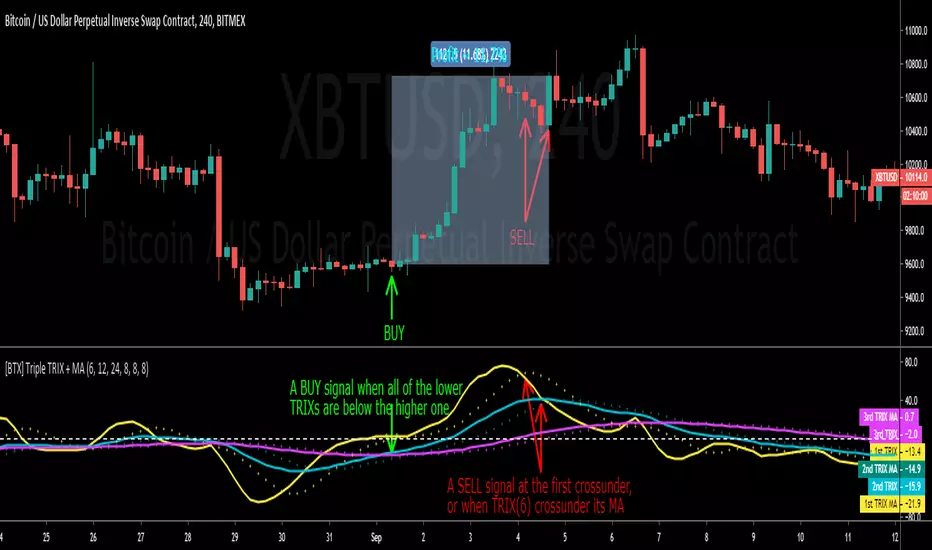
Fib,Guppy Multiple MA(FGMMA)(A/D & Volume Weight,SMA,EMA)[cI8DH]Features:
- 3 + 12 MAs (12 is chosen because Guppy has 12 MAs)
- MA types can be set to Simple, Exponential, Weighted, and Smoothed
- Volume weight can be applied to all available MAs (the built-in VWMA uses Simple MA)
- It is possible to count in only effective portions of the volume in the equation by using Accum/Dist Volume Weight
- Secondary smoothing (useful when volume weight is enabled)
- Predefined MA sets based on Fibonacci sequence (2,3,5,8,.., 377), Guppy (3,5,8,10,12,15 &30,35,40,45,50,60), and cI8DH (2,3,5,8,12,17 & 30,34,39,45,52,60)
Recommended settings:
- hlc3 as input source captures all the essential information encapsulated in a candle. I'd use hlc3 as the default option. In uptrend, "low" and in downtrend, "high" might give more relevant results when using MAs for structural analysis of a market. For commonly used MAs (EMA20, SMA50,100,200), "close" should be used due to their self-fulfilling prophecy effect.
- When you have volume weight above 0, you may want to use secondary smoothing.
- Try not to use Simple MA for smaller lengths (below 20). Sharp changes in the past (right before the period specified by the length) will affect the current value of MA dramatically leading to confusion.
- I am using the first 3 MAs for SMA 50,100,200. You can disable them from the MA type selector all at once when using Fib or Guppy ribbons.
MA-based analysis:
There are different ways of structuring a market. Geometrical (trend lines, channels, fans, patterns, etc) and Fib retracement-based structuring is very common among traders. MAs give an alternative way of analyzing markets. MA ribbons such as Guppy (6 slow and 6 fast-moving MAs) are popular for analyzing market flow. IMO default Guppy sets are a bit random as the numbers do not have an elegant sequence. So I proposed my sets based on increasing sequene spacing (+1). These two MA ribbons are good for market flow analysis but the spacing of the MAs are not ideal for structuring a market. Ribbons based on the Fib sequence is a better choice for structuring a market. This is the equivalent of Fib channels but in a more dynamic form. Among other things, MA Fib ribbon can be used to assess market momentum and to compare different stages of a market. Here are two "educational-only" examples:
Notes:
- Smoothed MA with length L = Exponential MA with length 2*L-1
- Read the background section in my ADP indicator to understand how A/D Volume is calculated

XPloRR MA-Trailing-Stop StrategyXPloRR MA-Trailing-Stop Strategy
Long term MA-Trailing-Stop strategy with Adjustable Signal Strength to beat Buy&Hold strategy
None of the strategies that I tested can beat the long term Buy&Hold strategy. That's the reason why I wrote this strategy.
Purpose: beat Buy&Hold strategy with around 10 trades. 100% capitalize sold trade into new trade.
My buy strategy is triggered by the fast buy EMA (blue) crossing over the slow buy SMA curve (orange) and the fast buy EMA has a certain up strength.
My sell strategy is triggered by either one of these conditions:
the EMA(6) of the close value is crossing under the trailing stop value (green) or
the fast sell EMA (navy) is crossing under the slow sell SMA curve (red) and the fast sell EMA has a certain down strength.
The trailing stop value (green) is set to a multiple of the ATR(15) value.
ATR(15) is the SMA(15) value of the difference between the high and low values.
The scripts shows a lot of graphical information:
The close value is shown in light-green. When the close value is lower then the buy value, the close value is shown in light-red. This way it is possible to evaluate the virtual losses during the trade.
the trailing stop value is shown in dark-green. When the sell value is lower then the buy value, the last color of the trade will be red (best viewed when zoomed)(in the example, there are 2 trades that end in gain and 2 in loss (red line at end))
the EMA and SMA values for both buy and sell signals are shown as a line
the buy and sell(close) signals are labeled in blue
How to use this strategy?
Every stock has it's own "DNA", so first thing to do is tune the right parameters to get the best strategy values voor EMA , SMA, Strength for both buy and sell and the Trailing Stop (#ATR).
Look in the strategy tester overview to optimize the values Percent Profitable and Net Profit (using the strategy settings icon, you can increase/decrease the parameters)
Then keep using these parameters for future buy/sell signals only for that particular stock.
Do the same for other stocks.
Important : optimizing these parameters is no guarantee for future winning trades!
Here are the parameters:
Fast EMA Buy: buy trigger when Fast EMA Buy crosses over the Slow SMA Buy value (use values between 10-20)
Slow SMA Buy: buy trigger when Fast EMA Buy crosses over the Slow SMA Buy value (use values between 30-100)
Minimum Buy Strength: minimum upward trend value of the Fast SMA Buy value (directional coefficient)(use values between 0-120)
Fast EMA Sell: sell trigger when Fast EMA Sell crosses under the Slow SMA Sell value (use values between 10-20)
Slow SMA Sell: sell trigger when Fast EMA Sell crosses under the Slow SMA Sell value (use values between 30-100)
Minimum Sell Strength: minimum downward trend value of the Fast SMA Sell value (directional coefficient)(use values between 0-120)
Trailing Stop (#ATR): the trailing stop value as a multiple of the ATR(15) value (use values between 2-20)
Example parameters for different stocks (Start capital: 1000, Order=100% of equity, Period 1/1/2005 to now) compared to the Buy&Hold Strategy(=do nothing):
BEKB(Bekaert): EMA-Buy=12, SMA-Buy=44, Strength-Buy=65, EMA-Sell=12, SMA-Sell=55, Strength-Sell=120, Stop#ATR=20
NetProfit: 996%, #Trades: 6, %Profitable: 83%, Buy&HoldProfit: 78%
BAR(Barco): EMA-Buy=16, SMA-Buy=80, Strength-Buy=44, EMA-Sell=12, SMA-Sell=45, Strength-Sell=82, Stop#ATR=9
NetProfit: 385%, #Trades: 7, %Profitable: 71%, Buy&HoldProfit: 55%
AAPL(Apple): EMA-Buy=12, SMA-Buy=45, Strength-Buy=40, EMA-Sell=19, SMA-Sell=45, Strength-Sell=106, Stop#ATR=8
NetProfit: 6900%, #Trades: 7, %Profitable: 71%, Buy&HoldProfit: 2938%
TNET(Telenet): EMA-Buy=12, SMA-Buy=45, Strength-Buy=27, EMA-Sell=19, SMA-Sell=45, Strength-Sell=70, Stop#ATR=14
NetProfit: 129%, #Trade

Back to zero: Understanding seriestype: pine series basic example
time required: 10 minutes
level: medium (need to know the "array" data variable as a generic programming concept, basic Pine syntax)
tl;dr how variables and series work in Pine
Pine is an array/vector language. That's something that twists how it behaves, and how we have to think about it. A lot of misunderstandings come from forgetting this fact. This example tries to clear that concept.
First, you need to know what an array is, and how it works in a programmig language. Also, having javascript under your belt helps too. If you don't, google "javascript array basic tutorial" is your friend :)
So, in pine arrays are called "series". Every variable is an array with values for each candle in the chart. if we do:
myVar = true
this is not a constant. It is a series of values for each candle, { true, true,....., true }
In practice, the result is the same, but we can access each of the values in the series, like myVar{0}, myVar{7}, myVar{anyNumber}....
Again, it is not a constant, since you can access/modify the each value individually
so, lets show it:
plot (myVar, clolor = gray)
this plots an horizontal line of value 1 ( 1 is equal to true ) so it's all good.
On to a more usual series:
tipicalSeries = close > open ? true : false
plot(tipicalSeries, color= blue)
This gives the expected result, a tipical up and down line with values at 1 or 0. Naturally, "tipicalSeries" is an array, the "ups" and "downs" are all stored under the same variable, indexed by the candles.
In Pine, the ZERO position in the array is the last one, which corresponds to the last candle on the right. Say you have a chart with 12 candles. The close would be the closing value of what we intuitively think as first candle, the one on the left. then close ... and so on.... until close , the value of the "last" candle, the one on the right. It actually helps to start thinking of the positions backwards, counting down to zero, rocket launch style :)
And back to our series. The myVar will also be the same size, from myVar to myVar .
When we do some operation with them, something simple like
if ( myVar == tipicalSeries)
what is really happening is that internally, Pine is checking each of the indexes, as in myVar == tipicalSeries , myVar == tipicalSeries .... myVar == tipicalSeries
And we can store that stuff to check it. simply:
result = (myVar == tipicalSeries) ? true : false //yes, this is the same as tipicalSeries, but we're not in a boolean logic tut ;)
plot (result)
The reason we can plot the result is that it is an array, not a single value. The example indicator i provide shows a plot where the values are obtained from different places in the array, this line here:
mySeries3 = mySeries2 and mySeries1
this creates a series that is the result of the PREVIOUS values stored (the zero index is the one most at the right, or the "current" one), which here just causes a shift in the plotted line by one candle.
Go ahead, grab a copy of my code, try to change the indexes and see the results. Understanding this stuff is critical to go deeper into Pine :)

CRAZY RAY RAY - Dashboard 1-5-15-1D + SMC + Clock + Candles PRO OANDA:XAUUSD This script is essentially your institutional "nuclear power plant" for scalping and swing trading: it combines the 1-5-15-1D dashboard, SMC, PRO candles, money flow times, institutional filters, Bull/Bear 12C, Liquidity HUD, Fibo Move, and Target Trend with SL + 3 TPs into a single indicator. 1. Dashboard 1–5–15–1D (Central HUD)
Calculates across 4 timeframes: 1m, 5m, 15m, and 1D:
Trend with EMAs 15/30/200.
RSI (strength >50 buy, <50 sell).
MACD (crossover in favor or against).
For each timeframe it shows:
TREND → BULLISH / BEARISH / NEUTRAL.
ACTION → BUY / SELL / WAIT.
If all 4 timeframes align:
MODE = BULLISH BUY
MODE = BEARISH SELL
Filters and displays on the HUD if buys or sells are blocked by SMC context (BLOCKED BUY / BLOCKED SELL).
Also draws 2 simple moving averages on the chart:
SMA 20 white (you can use it as a micro-trend).
SMA 200 red (macro trend and institutional reference).
2. Real-Time Clock + Trading Hours
Calculates the real time for:
New York / Miami
London
Tokyo
using current time and real time zone.
Also calculates GMT time to know which session is dominant.
Marks your trading hours:
LONDON 3:00–5:30 (London time) → goodLondon
NY OPEN 8:30–10:00 (NY time) → goodNYOpen
ASIA 20:00–23:00 (Tokyo) → goodAsiaScalp
Displays a message on the HUD:
LONDON 3:00–5:30 (1–2 TRADES)
NY OPEN 8:30–10:00 (1 TRADE)
ASIA 20–23 (SCALP)
NO TRADE ROLL / DEAD / LATE
ONLY A+ SETUPS (when not in strong trading hours).
3. Institutional Power (volume + ATR + session)
Filter that evaluates whether the moment is institutional or retail:
Checks:
If you are in a strong trading session (London / NY). If the volume is above the average × multiplier.
If the ATR is above the average × multiplier.
If it passes the filters → INST ON, otherwise → RETAIL ZONE.
Used internally to block buys/sells and for the HUD.
4. Micro-signal “NO RETRACEMENT” on 1m (BUY SR / SELL SR)
On the 1-minute timeframe, it detects a very aggressive entry:
Clean trend (15/30/200 EMAs aligned).
Price crosses the 200 EMA.
MACD turns in favor.
Marks on the candle:
BUY SR (buys without retracement below the EMA200).
SELL SR (sales without retracement above the EMA200).
This state is also reflected in the HUD as the “SR” row.
5. SMC Block: HH/HL/LH/LL + BMS + ChoCH + Fibo + Zones
This is the SMC brain of the script:
Detects swings with pivots:
Paints HH, HL, LH, LL (if you activate showHHLL).
Marks BOS (break of structure).
Marks BMS and ChoCH (with strong or weak filter using ATR, volume, MACD, gaps).
Draws:
Internal Fibo of the last range (38–50–61).
Fibo entry zone 38–78% as a green discount/premium box.
Institutional mitigation zones (simple OB type green/red boxes).
Current range with dotted yellow lines.
Calculates logic for:
antiStupidBuy: blocks purchases when the context is very bearish (LL–LL–LH, bearish ChoCH, premium, EQH, etc.).
antiStupidSell: symmetrical for sales.
From this comes:
allowBuyInst
allowSellInst
buyBlockerOn / sellBlockerOn
buyTrapDetected (BUY SR signal but context blocks it → BUY TRAP).
All this feeds the HUD and institutional alerts.
6. PRO Candles (candlestick + smart color)
Candlestick pattern system:
Detects:
Hammer, Inverted Hammer. Doji.
Strong bullish/bearish candle.
Bullish/bearish engulfing.
Uses a trend EMA to determine if the pattern is with or against the trend.
Colors the candles according to the pattern (if you enable useColorCandles).
Defines texts:
patternText (pattern name).
biasText (reversal, momentum, indecision).
Updates the HUD with the current pattern (“CANDLE: Engulf Bull”, etc.).
7. Institutional PRO Combo + Reversals
Connects everything:
fullBuySetup:
allowBuyInst TRUE (SMC + Fibo + mitigation OK).
Institutional candles in favor (engulfing, hammer, etc.).
MultiTF aligned (1m, 5m in favor, 15/1D not strongly against).
Strong session (London or NY).
No blockages.
fullSellSetup: the same for sales.
Marks on the chart:
BUY PRO, SELL PRO.
BUY REV LL → reversal from a LL, at Fibo discount, with an institutional candle and above EMA200.
SELL REV HH → reversal from HH, at Fibo premium, with an institutional candle and below EMA200.
And generates alerts for all of this.
8. Dynamic Main HUD
On barstate.islast, updates the HUD:
Changes “BUY / SELL” to:
BUY BLOCK / SELL BLOCK when the context blocks that direction.
Writes:
Current candle pattern.
Time message.
Global status:
BUY TRAP ❌, BUY REV LL ✅, SELL REV HH ✅, BUY PRO ✅, SELL PRO ✅,
BUY BLOCK, SELL BLOCK, BUY/SELL OK.
9. Bull/Bear 12C HUD (Small right HUD)
12-confirmation bull/bear engine:
Calculates:
Sweep, 5th leg, mitigation, HL/LH, strong BOS.
Volume pattern (high-low-high).
ATR rising.
MACD crossover.
Liquidity.
Fear & Greed (SMA50).
Gap/imbalance. Bull/Bear 180 weak.
Count how many are ON:
bullScore /12
bearScore /12
Define a regime:
INSTITUTIONAL → many confirmations + rvol + ATR.
NORMAL
RETAIL
Show on right HUD:
List 1 to 12 with green/red dots BULL / BEAR.
Summary: “Regime: INSTITUTIONAL / NORMAL / RETAIL”.
10. Liquidity HUD XAU SCALP
Calculates RVOL, normalized ATR, spread vs ATR, current range vs average range.
Generates score and classifies:
LOW / MED / HIGH / INS.
Only moves up one level if you are in London/NY session (depending on sessions)

ACCDv3# ACCDv3 - Accumulation/Distribution MACD with Divergence Detection
## Overview
**ACCDv3** (Accumulation/Distribution MACD Version 3) is an advanced volume-weighted momentum indicator that combines the Accumulation/Distribution (A/D) line with MACD methodology and divergence detection. It helps identify trend strength, momentum shifts, and potential reversals by analyzing volume-weighted price movements.
## Key Features
- **Volume-Weighted MACD**: Applies MACD calculation to volume-weighted A/D values for earlier, more reliable signals
- **Divergence Detection**: Identifies when A/D trend diverges from MACD momentum
- **Volume Strength Filtering**: Distinguishes high-volume confirmations from low-volume noise
- **Color-Coded Histogram**: 4-color system showing momentum direction and volume strength
- **Real-Time Alerts**: Background colors and alert conditions for bullish/bearish divergences
## Components
### 1. Accumulation/Distribution (A/D) Line
The A/D line measures buying and selling pressure by comparing the close price to the trading range, weighted by volume:
```
A/D = Σ ((2 × Close - Low - High) / (High - Low)) × Volume
```
- **Rising A/D**: More accumulation (buying pressure)
- **Falling A/D**: More distribution (selling pressure)
- **Doji Handling**: When High = Low, contribution is zero (avoids division errors)
### 2. Volume-Weighted MACD
Instead of simple EMAs, the indicator weights A/D values by volume:
- **Fast Line** (default 12): `EMA(A/D × Volume, 12) / EMA(Volume, 12)`
- **Slow Line** (default 26): `EMA(A/D × Volume, 26) / EMA(Volume, 26)`
- **MACD Line**: Fast Line - Slow Line (green line)
- **Signal Line** (default 9): EMA or SMA of MACD (orange line)
- **Histogram**: MACD - Signal (color-coded columns)
This volume-weighting ensures that periods with higher volume have greater influence on the indicator values.
### 3. Histogram Color System
The histogram uses 4 distinct colors based on **direction** and **volume strength**:
| Condition | Color | Meaning |
|-----------|-------|---------|
| Rising + High Volume | **Dark Green** (#1B5E20) | Strong bullish momentum with volume confirmation |
| Rising + Low Volume | **Light Teal** (#26A69A) | Bullish momentum but weak volume (less reliable) |
| Falling + High Volume | **Dark Red** (#B71C1C) | Strong bearish momentum with volume confirmation |
| Falling + Low Volume | **Light Red/Pink** (#FFCDD2) | Bearish momentum but weak volume (less reliable) |
Additional shading:
- **Light Cyan** (#B2DFDB): Positive but not rising (momentum stalling)
- **Bright Red** (#FF5252): Negative and accelerating down
### 4. Divergence Detection
Divergence occurs when A/D trend and MACD momentum move in opposite directions:
#### Bullish Divergence (Green Background)
- **Condition**: A/D is trending up BUT MACD is negative and trending down
- **Interpretation**: Accumulation increasing while momentum appears weak
- **Signal**: Potential bullish reversal or continuation
- **Action**: Look for entry opportunities or hold long positions
#### Bearish Divergence (Red Background)
- **Condition**: A/D is trending down BUT MACD is positive and trending up
- **Interpretation**: Distribution increasing while momentum appears strong
- **Signal**: Potential bearish reversal or weakening uptrend
- **Action**: Consider exits, tighten stops, or prepare for reversal
## Parameters
| Parameter | Default | Range | Description |
|-----------|---------|-------|-------------|
| **Fast Length** | 12 | 1-50 | Period for fast EMA (shorter = more sensitive) |
| **Slow Length** | 26 | 1-100 | Period for slow EMA (longer = smoother) |
| **Signal Smoothing** | 9 | 1-50 | Period for signal line (MACD smoothing) |
| **Signal Line MA Type** | EMA | SMA/EMA | Moving average type for signal calculation |
| **Volume MA Length** | 20 | 5-100 | Period for volume average (strength filter) |
## Usage Guide
### Reading the Indicator
1. **MACD Lines (Green & Orange)**
- **Crossovers**: When green crosses above orange = bullish, below = bearish
- **Distance**: Wider gap = stronger momentum
- **Zero Line**: Above = bullish bias, below = bearish bias
2. **Histogram Colors**
- Focus on **dark colors** (dark green/red) for high-confidence signals
- Be cautious with **light colors** (teal/pink) - wait for volume confirmation
- Watch for **rising red bars** (V-bottom pattern) = potential bullish reversal
- Watch for **falling green bars** (Λ-top pattern) = potential bearish reversal
3. **Background Divergence Alerts**
- **Green background**: Bullish divergence - consider long entries
- **Red background**: Bearish divergence - consider exits or shorts
- Best used in combination with price action and support/resistance levels
### Trading Strategies
#### Trend Following
1. Wait for MACD to cross above zero line with dark green histogram
2. Enter long when histogram shows consecutive dark green bars
3. Exit when histogram turns light green or red appears
#### Divergence Trading
1. Wait for background divergence alert (green or red)
2. Confirm with price action (support/resistance, candlestick patterns)
3. Enter on next dark-colored histogram bar in divergence direction
4. Set stops beyond recent swing high/low
#### Volume Confirmation
1. Ignore signals during low-volume periods (light colors)
2. Take aggressive positions during high-volume confirmations (dark colors)
3. Use volume strength as position sizing guide (larger size on dark bars)
### Best Practices
✓ **Combine with price action**: Don't rely on indicator alone
✓ **Wait for dark colors**: High-volume bars are more reliable
✓ **Watch for divergences**: Early warning signs of reversals
✓ **Use multiple timeframes**: Confirm signals across 1m, 5m, 15m
✓ **Respect zero line**: Trading direction should align with MACD side
✗ **Don't chase light-colored signals**: Low volume = lower reliability
✗ **Don't ignore context**: Market structure and levels matter
✗ **Don't over-trade**: Wait for clear, high-volume setups
✗ **Don't ignore alerts**: Divergences are early warnings
## Technical Details
### Volume-Weighted Calculation Method
Traditional MACD uses simple price EMAs. ACCDv3 weights each A/D value by its corresponding volume:
```pine
// Volume-weighted fast EMA
close_vol_fast = ta.ema(ad × volume, fast_length)
vol_fast = ta.ema(volume, fast_length)
vw_ad_fast = close_vol_fast / vol_fast
// Same for slow EMA
close_vol_slow = ta.ema(ad × volume, slow_length)
vol_slow = ta.ema(volume, slow_length)
vw_ad_slow = close_vol_slow / vol_slow
// MACD is the difference
macd = vw_ad_fast - vw_ad_slow
```
This ensures high-volume periods have proportionally more impact on the indicator.
### Volume Strength Filter
Determines whether current volume is above or below average:
```pine
vol_avg = ta.sma(volume, vol_length)
vol_strength = volume > vol_avg
```
Used to select dark (high volume) vs light (low volume) histogram colors.
### Divergence Logic
```pine
// A/D trending up if above its 5-period SMA
ad_trend = ad > ta.sma(ad, 5)
// MACD trending up if above zero
macd_trend = macd > 0
// Divergence when trends oppose
divergence = ad_trend != macd_trend
// Specific conditions
bullish_divergence = ad_trend and not macd_trend and macd < 0
bearish_divergence = not ad_trend and macd_trend and macd > 0
```
## Alerts
The indicator includes built-in alert conditions:
- **Bullish Divergence**: "Bullish Divergence: A/D trending up but MACD trending down"
- **Bearish Divergence**: "Bearish Divergence: A/D trending down but MACD trending up"
To enable:
1. Click "Create Alert" button in TradingView
2. Select "ACCDv3" as condition
3. Choose "Bullish Divergence" or "Bearish Divergence"
4. Configure notification method (popup, email, webhook, etc.)
## Comparison with Standard MACD
| Feature | Standard MACD | ACCDv3 |
|---------|---------------|---------|
| **Input** | Close price | Accumulation/Distribution line |
| **Weighting** | Simple EMA | Volume-weighted EMA |
| **Divergence** | Price vs MACD | A/D vs MACD |
| **Volume Analysis** | None | Built-in strength filter |
| **Color System** | 2 colors (up/down) | 4+ colors (direction + volume) |
| **Leading/Lagging** | Lagging | More leading (volume-weighted) |
## Example Scenarios
### Scenario 1: Strong Bullish Signal
- **Chart**: MACD crosses above zero line
- **Histogram**: Dark green bars (#1B5E20) appearing
- **Volume**: Above 20-period average
- **Action**: Enter long, strong momentum with volume confirmation
### Scenario 2: Weak Bearish Signal
- **Chart**: MACD crosses below zero line
- **Histogram**: Light pink bars (#FFCDD2) appearing
- **Volume**: Below 20-period average
- **Action**: Avoid shorting, low volume = unreliable signal
### Scenario 3: Bullish Divergence Reversal
- **Chart**: Price making lower lows
- **Indicator**: A/D line trending up, MACD negative
- **Background**: Green shading appears
- **Histogram**: Transitions from red to dark green
- **Action**: Look for long entry on next dark green bar
### Scenario 4: V-Bottom Reversal
- **Chart**: Downtrend in place
- **Histogram**: Red bars start rising (becoming less negative)
- **Pattern**: Forms "V" shape at bottom
- **Confirmation**: Transitions to dark green bars
- **Action**: Bullish reversal signal, consider long entry
## Timeframe Recommendations
- **1-minute**: Scalping, very fast signals (noisy, use with caution)
- **5-minute**: Intraday momentum trading (recommended)
- **15-minute**: Swing entries, clearer trend signals
- **1-hour+**: Position trading, major trend identification
## Limitations
- **Requires volume data**: Will not work on instruments without volume
- **Lag during consolidation**: MACD is inherently trend-following
- **False signals in chop**: Sideways markets generate noise
- **Not a standalone system**: Should be combined with price action and risk management
## Version History
- **v3**: Removed traditional price MACD, using only volume-weighted A/D MACD with A/D divergence
- **v2**: Added A/D divergence detection, volume strength filtering, enhanced histogram colors
- **v1**: Basic MACD on A/D line with volume-weighted calculation
## Support & Further Reading
For questions, updates, or to report issues, refer to the main project documentation or contact the developer.
**Related Indicators in Suite:**
- **VMACDv3**: Volume-weighted MACD on price (not A/D)
- **RSIv2**: RSI with A/D divergence
- **DMI**: Directional Movement Index with A/D divergence
- **Elder Impulse**: Bar coloring system using volume-weighted MACD
---
*This indicator is for educational purposes. Always practice proper risk management and never risk more than you can afford to lose.*

YM Ultimate SNIPER v5# YM Ultimate SNIPER v5 - Documentation & Trading Guide
## 🎯 Unified GRA + DeepFlow | YM/MYM Optimized
**TARGET: 3-7 High-Confluence Trades per Day**
---
## ⚡ QUICK START
```
┌─────────────────────────────────────────────────────────────────┐
│ YM ULTIMATE SNIPER v5 │
├─────────────────────────────────────────────────────────────────┤
│ │
│ SIGNALS: │
│ S🎯 = S-Tier (50+ pts) → HOLD position │
│ A🎯 = A-Tier (25-49 pts) → SWING trade │
│ B🎯 = B-Tier (12-24 pts) → SCALP quick │
│ Z = Zone entry (price at FVG zone) │
│ │
│ SESSIONS (ET): │
│ LDN = 3:00-5:00 AM (London) │
│ NY = 9:30-11:30 AM (New York Open) │
│ PWR = 3:00-4:00 PM (Power Hour) │
│ │
│ COLORS: │
│ 🟩 Green zones = Bullish FVG (buy zone) │
│ 🟥 Red zones = Bearish FVG (sell zone) │
│ 🟣 Purple lines = Single prints (S/R levels) │
│ │
│ TABLE (Top Right): │
│ Pts = Candle point range │
│ Tier = S/A/B/X classification │
│ Vol = Volume ratio (green = good) │
│ Delta = Buy/Sell dominance │
│ Sess = Current session │
│ Zone = In FVG zone status │
│ Score = Confluence score /10 │
│ CVD = Cumulative delta direction │
│ R:R = Risk:Reward ratio │
│ │
└─────────────────────────────────────────────────────────────────┘
```
---
## 📋 VERSION 5 CHANGES
### What's New
- **Removed all imbalance code** - caused compilation errors
- **Simplified delta analysis** - uses candle structure instead of intrabar data
- **Cleaner confluence scoring** - 5 clear factors, max 10 points
- **Reliable table** - updates on last bar only, no flickering
- **Works on YM and MYM** - same logic applies to micro contracts
### Removed Features
- Candle-anchored imbalance markers
- Imbalance S/R zones
- Intrabar volume profile analysis
- POC visualization
### Kept & Improved
- Tier classification (S/A/B)
- FVG zone detection & visualization
- Single print detection
- Session windows with backgrounds
- Confluence scoring
- Stop/Target auto-calculation
- All alerts
---
## 🎯 SIGNAL TYPES
### Tier Signals (S🎯, A🎯, B🎯)
These are high-confluence signals that pass all filters:
| Tier | Points | Value/Contract | Action | Hold Time |
|------|--------|----------------|--------|-----------|
| **S** | 50+ | $250+ | HOLD | 2-5 min |
| **A** | 25-49 | $125-245 | SWING | 1-3 min |
| **B** | 12-24 | $60-120 | SCALP | 30-90 sec |
**Filters Required:**
1. Tier threshold met (points)
2. Volume ≥ 1.8x average
3. Delta dominance ≥ 62%
4. Body ratio ≥ 70%
5. Range ≥ 1.3x average
6. Proper wicks (no reversal wicks)
7. CVD confirmation (optional)
8. In trading session
### Zone Signals (Z)
Zone entries trigger when:
- Price is inside an FVG zone
- Delta shows dominance in zone direction
- Volume is above average
- In active session
- No tier signal already present
---
## 📊 CONFLUENCE SCORING
**Maximum Score: 10 points**
| Factor | Points | Condition |
|--------|--------|-----------|
| Tier | 1-3 | B=1, A=2, S=3 |
| In Zone | +2 | Price inside FVG zone |
| Strong Volume | +2 | Volume ≥ 2x average |
| Strong Delta | +2 | Delta ≥ 70% |
| CVD Momentum | +1 | CVD trending with signal |
**Score Interpretation:**
- **7-10**: Elite setup - full size
- **5-6**: Good setup - standard size
- **4**: Minimum threshold - reduced size
- **< 4**: No signal shown
---
## ⏰ SESSION WINDOWS
### London (3:00-5:00 AM ET)
- European institutional flow
- Character: Slow build-up, clean trends
- Expected trades: 1-2
- Best for: Zone entries, A/B tier
### NY Open (9:30-11:30 AM ET)
- Highest volume, most institutional activity
- Character: Initial balance, breakouts
- Expected trades: 2-3
- Best for: S/A tier, zone confluence
### Power Hour (3:00-4:00 PM ET)
- End-of-day rebalancing, MOC orders
- Character: Mean reversion or trend acceleration
- Expected trades: 1-2
- Best for: Zone entries, B tier scalps
---
## 🟩 FVG ZONES
### What Are FVG Zones?
Fair Value Gaps (FVGs) are price gaps between candles where price moved so fast that a gap was left. These gaps often act as support/resistance.
### Zone Requirements
- Gap size ≥ 25% of ATR
- Impulse candle has strong body (≥ 70%)
- Impulse candle is 1.5x average range
- Volume above average on impulse
- Created during active session
### Zone States
1. **Fresh** (bright color) - Just created, untested
2. **Tested** (gray) - Price touched zone midpoint
3. **Broken** (removed) - Price closed through zone
### Trading FVG Zones
| Zone | Approach From | Expected |
|------|--------------|----------|
| 🟩 Bull | Above (falling) | Support - look for bounce |
| 🟥 Bear | Below (rising) | Resistance - look for rejection |
---
## 🟣 SINGLE PRINTS
Single prints mark candles with:
- Range > 1.3x average
- Body > 70% of range
- Volume > 1.8x average
- Clear delta dominance
These become horizontal support/resistance lines extending into the future.
---
## 📊 TABLE REFERENCE
| Row | Label | Meaning |
|-----|-------|---------|
| 1 | Pts | Current candle point range |
| 2 | Tier | S/A/B/X classification |
| 3 | Vol | Volume ratio vs 20-bar average |
| 4 | Delta | Buy/Sell percentage dominance |
| 5 | Sess | Current session (LDN/NY/PWR/OFF) |
| 6 | Zone | In FVG zone (BULL/BEAR/---) |
| 7 | Score | Confluence score out of 10 |
| 8 | CVD | Delta momentum direction |
| 9 | R:R | Risk:Reward if signal active |
### Color Coding
- **Green/Lime**: Good, meets threshold
- **Yellow**: Caution, borderline
- **Red**: Bad, below threshold
- **Gray**: Inactive/neutral
---
## 🔧 SETTINGS GUIDE
### Tier Thresholds
| Setting | Default | Notes |
|---------|---------|-------|
| S-Tier | 50 pts | ~$250/contract |
| A-Tier | 25 pts | ~$125/contract |
| B-Tier | 12 pts | ~$60/contract |
### Sniper Filters
| Setting | Default | Notes |
|---------|---------|-------|
| Min Volume Ratio | 1.8x | Lower = more signals |
| Delta Dominance | 62% | Lower = more signals |
| Body Ratio | 70% | Higher = fewer, cleaner |
| Range Multiplier | 1.3x | Higher = fewer, bigger moves |
| CVD Confirm | On | Off = more signals |
### Recommended Configurations
**Conservative (3-4 trades/day):**
```
Min Confluence: 6
Volume Ratio: 2.0
Delta Threshold: 65%
Body Ratio: 75%
```
**Standard (5-7 trades/day):**
```
Min Confluence: 4
Volume Ratio: 1.8
Delta Threshold: 62%
Body Ratio: 70%
```
**Aggressive (7-10 trades/day):**
```
Min Confluence: 3
Volume Ratio: 1.5
Delta Threshold: 60%
Body Ratio: 65%
```
---
## ✓ ENTRY CHECKLIST
Before entering any trade:
1. ☐ Signal present (S🎯, A🎯, B🎯, or Z)
2. ☐ Session active (LDN, NY, or PWR)
3. ☐ Score ≥ 4 (preferably 6+)
4. ☐ Vol shows GREEN
5. ☐ Delta colored (not gray)
6. ☐ CVD arrow matches direction
7. ☐ Note stop/target lines
8. ☐ Execute at signal candle close
---
## ⛔ DO NOT TRADE
- Session shows "OFF"
- Score < 4
- Vol shows RED
- Delta gray (no dominance)
- Multiple conflicting signals
- Major news imminent (FOMC, NFP, CPI)
- Overnight session (11:30 PM - 3:00 AM ET)
---
## 🎯 POSITION SIZING
| Tier | Score | Size | Stop |
|------|-------|------|------|
| S (50+ pts) | 7+ | 100% | Below/above candle |
| A (25-49 pts) | 5-6 | 75% | Below/above candle |
| B (12-24 pts) | 4 | 50% | Below/above candle |
| Zone | Any | 50% | Beyond zone |
---
## 🚨 ALERTS
### Priority Alerts (Set These)
| Alert | Action |
|-------|--------|
| 🎯 S-TIER | Drop everything, check immediately |
| 🎯 A-TIER | Evaluate within 15 seconds |
| 🎯 B-TIER | Check if available |
| 🎯 ZONE | Good context entry |
### Info Alerts (Optional)
| Alert | Purpose |
|-------|---------|
| NEW BULL/BEAR FVG | Mark zones on mental map |
| SINGLE PRINT | Note for future S/R |
| SESSION OPEN | Prepare to trade |
---
## 📈 TRADE JOURNAL
```
DATE: ___________
SESSION: ☐ LDN ☐ NY ☐ PWR
TRADE:
├── Time: _______
├── Signal: S🎯 / A🎯 / B🎯 / Z
├── Direction: LONG / SHORT
├── Score: ___/10
├── Entry: _______
├── Stop: _______
├── Target: _______
├── In Zone: ☐ Yes ☐ No
├── Result: +/- ___ pts ($_____)
└── Notes: _______________________
DAILY:
├── Trades: ___
├── Wins: ___ | Losses: ___
├── Net P/L: $_____
└── Best setup: _______________________
```
---
## 🏆 GOLDEN RULES
> **"Wait for the session. Off-hours = noise."**
> **"Score 6+ is your edge. Anything less is gambling."**
> **"Zone + Tier = bread and butter combo."**
> **"One great trade beats five forced trades."**
> **"Leave every trade with money. YM gives you time."**
---
## 🔧 TROUBLESHOOTING
| Issue | Solution |
|-------|----------|
| No signals | Lower min score to 3-4 |
| Too many signals | Raise min score to 6+ |
| Zones cluttering | Reduce max zones to 8 |
| Missing sessions | Check timezone setting |
| Table not updating | Resize chart or refresh |
---
## 📝 TECHNICAL NOTES
- **Pine Script v6**
- **Works on**: YM, MYM, any Dow futures
- **Recommended TF**: 1-5 minute for day trading
- **Min TradingView Plan**: Free (no intrabar data required)
---
*© Alexandro Disla - YM Ultimate SNIPER v5*
*Clean Build | Proven Components Only*

YM Ultimate SNIPER# YM Ultimate SNIPER - Documentation & Trading Guide
## 🎯 Unified GRA + DeepFlow | YM-Optimized for Low Volatility
**TARGET: 3-7 High-Confluence Trades per Day**
> **Philosophy:** *YM's lower volatility is not a weakness—it's our edge. Predictability + precision = consistent profits.*
---
## ⚡ QUICK REFERENCE CARD
```
┌─────────────────────────────────────────────────────────────────────────────┐
│ YM ULTIMATE SNIPER - QUICK REFERENCE │
├─────────────────────────────────────────────────────────────────────────────┤
│ │
│ 💰 YM BASICS: │
│ ═════════════ │
│ • 1 tick = 1 point = $5/contract │
│ • Typical daily range: 150-400 points │
│ • 30-40% less volatile than NQ │
│ • More institutional, less retail noise │
│ │
├─────────────────────────────────────────────────────────────────────────────┤
│ │
│ 🎯 TIER THRESHOLDS (YM-OPTIMIZED): │
│ ══════════════════════════════════ │
│ S-TIER: 50+ pts = $250+/contract → HOLD (Institutional sweep) │
│ A-TIER: 25-49 pts = $125-245/contract → SWING (Strong momentum) │
│ B-TIER: 12-24 pts = $60-120/contract → SCALP (Quick grab) │
│ │
├─────────────────────────────────────────────────────────────────────────────┤
│ │
│ ⏰ SESSION WINDOWS: │
│ ═══════════════════ │
│ LDN → 3:00-5:00 AM ET (European flow) │
│ NY → 9:30-11:30 AM ET (US opening drive) │
│ PWR → 3:00-4:00 PM ET (End-of-day rebalancing) │
│ │
│ Expected Trades: 1-2 LDN | 2-3 NY | 1-2 PWR = 4-7 total │
│ │
├─────────────────────────────────────────────────────────────────────────────┤
│ │
│ 📊 CONFLUENCE SCORING (MAX 10 POINTS): │
│ ═══════════════════════════════════════ │
│ Tier Signal: S=3, A=2, B=1 points │
│ In Active Zone: +2 points │
│ POC Aligned: +1 point (POC at body extreme) │
│ Imbalance Support:+1 point (supporting IMB nearby) │
│ Strong Volume: +1 point (2x+ average) │
│ Strong Delta: +1 point (70%+ dominance) │
│ CVD Momentum: +1 point (CVD trending with signal) │
│ │
│ MINIMUM SCORE: 5/10 to show signal (adjustable) │
│ IDEAL SCORE: 7+/10 for highest probability │
│ │
├─────────────────────────────────────────────────────────────────────────────┤
│ │
│ 🚨 SIGNAL TYPES: │
│ ═════════════════ │
│ S🎯 / A🎯 / B🎯 → GRA Tier Signals (Full confluence) │
│ Z🎯 → Zone Entry (At DFZ zone + delta + volume) │
│ SP → Single Print (Institutional impulse) │
│ │
├─────────────────────────────────────────────────────────────────────────────┤
│ │
│ ✓ ENTRY CHECKLIST: │
│ ═══════════════════ │
│ □ Signal appears (check Score ≥5) │
│ □ Session active (LDN!/NY!/PWR!) │
│ □ Table: Vol GREEN, Delta colored, Body GREEN │
│ □ CVD arrow (▲/▼) matches direction │
│ □ Note stop/target lines on chart │
│ □ Check Zone status (bonus if IN ZONE) │
│ □ Execute at signal candle close │
│ │
├─────────────────────────────────────────────────────────────────────────────┤
│ │
│ 🎯 POSITION SIZING BY TIER: │
│ ═══════════════════════════ │
│ S-TIER (50+ pts): Full size, hold 2-5 min, target 2.5:1 R:R │
│ A-TIER (25-49): 75% size, hold 1-3 min, target 2.0:1 R:R │
│ B-TIER (12-24): 50% size, hold 30-90 sec, target 1.5:1 R:R │
│ │
├─────────────────────────────────────────────────────────────────────────────┤
│ │
│ ⛔ DO NOT TRADE WHEN: │
│ ════════════════════ │
│ ✗ Session shows "---" │
│ ✗ Score < 5/10 │
│ ✗ Vol shows RED (<1.8x) │
│ ✗ Delta < 62% │
│ ✗ Multiple conflicting signals │
│ ✗ Just before major news (FOMC, NFP, etc.) │
│ │
└─────────────────────────────────────────────────────────────────────────────┘
```
---
## 📋 WHY YM? LEVERAGING LOW VOLATILITY
### The YM Advantage
Most traders avoid YM because "it doesn't move enough." This is precisely why it's perfect for precision scalping:
| Factor | NQ | YM | Advantage |
|--------|----|----|-----------|
| **Daily Range** | 300-600 pts | 150-400 pts | More predictable moves |
| **Tick Value** | $5/tick (4 ticks/pt) | $5/tick (1 tick/pt) | Simpler math |
| **Retail Noise** | High | Low | Cleaner signals |
| **Whipsaws** | Frequent | Rare | Fewer fakeouts |
| **Trend Persistence** | Short | Long | Easier holds |
| **Fill Quality** | Variable | Consistent | Better execution |
### Why 3-7 Trades is the Sweet Spot
```
YM SESSION BREAKDOWN:
════════════════════
LONDON (3-5 AM ET): 1-2 trades
├── Why: European institutions positioning for US open
├── Character: Slow build-up, clean trends
└── Best signals: Zone entries + A/B tier
NY OPEN (9:30-11:30 AM ET): 2-3 trades
├── Why: Highest volume, most institutional activity
├── Character: Initial balance formation, breakouts
└── Best signals: S/A tier, zone confluence
POWER HOUR (3-4 PM ET): 1-2 trades
├── Why: End-of-day rebalancing, MOC orders
├── Character: Mean reversion or trend acceleration
└── Best signals: Zone entries, B tier quick scalps
TOTAL: 4-7 high-quality setups per day
```
---
## 🔧 YM-SPECIFIC OPTIMIZATIONS
This unified indicator has been specifically tuned for YM's characteristics:
### Tier Thresholds
| Tier | NQ (Original) | YM (Optimized) | Rationale |
|------|---------------|----------------|-----------|
| S-Tier | 100 pts | **50 pts** | YM's daily range is ~50% of NQ |
| A-Tier | 50 pts | **25 pts** | Proportional scaling |
| B-Tier | 20 pts | **12 pts** | Still 5%+ of typical daily range |
### Filter Adjustments
| Filter | NQ Value | YM Value | Why |
|--------|----------|----------|-----|
| Volume Ratio | 1.5x | **1.8x** | Higher bar = less retail noise |
| Delta Threshold | 60% | **62%** | Tighter for cleaner signals |
| Body Ratio | 70% | **72%** | More conviction required |
| Range Multiplier | 1.3x | **1.4x** | Bigger move = real signal |
| Gap ATR% | 30% | **25%** | Smaller gaps still significant |
| Zone Age | 50 bars | **75 bars** | Zones last longer in slow market |
### Why These Changes Work
1. **Higher Volume Bar**: YM has more institutional flow. Requiring 1.8x volume ensures we're catching real moves, not retail chop.
2. **Tighter Delta**: With less noise, we can demand clearer buyer/seller dominance before entering.
3. **Longer Zone Life**: YM trends persist longer. A zone that would be stale in NQ is still viable in YM.
4. **Smaller Gap Threshold**: YM gaps are naturally smaller. 25% of ATR in YM is significant institutional activity.
---
## 📊 CONFLUENCE SCORING SYSTEM
The unified indicator uses a 10-point confluence scoring system to filter for only the highest-probability setups:
### Score Breakdown
```
CONFLUENCE SCORE CALCULATION:
═════════════════════════════
BASE POINTS (Tier):
├── S-Tier signal: +3 points
├── A-Tier signal: +2 points
└── B-Tier signal: +1 point
BONUS POINTS:
├── Inside Active Zone (DFZ): +2 points
│ └── Price within bull/bear zone = institutional level
│
├── POC Alignment: +1 point
│ └── POC at body extreme = strong conviction
│
├── Imbalance Support: +1 point
│ └── Supporting imbalance within 1 ATR
│
├── Strong Volume (2x+): +1 point
│ └── Exceptional institutional participation
│
├── Strong Delta (70%+): +1 point
│ └── Clear one-sided aggression
│
└── CVD Momentum: +1 point
└── CVD trending with signal direction
MAXIMUM POSSIBLE: 10 points
```
### Score Interpretation
| Score | Quality | Action | Expected Win Rate |
|-------|---------|--------|-------------------|
| 8-10 | 🥇 Elite | Full size, hold for target | 75-80% |
| 6-7 | 🥈 Strong | Standard size, manage actively | 65-70% |
| 5 | 🥉 Valid | Reduced size, quick scalp | 55-60% |
| <5 | ⚫ Filtered | No signal shown | N/A |
### Adjusting Minimum Score
- **Conservative (Score ≥6)**: Fewer trades, higher win rate
- **Standard (Score ≥5)**: Balanced approach, 3-7 trades/day
- **Aggressive (Score ≥4)**: More trades, requires active management
---
## 📐 SIGNAL TYPES EXPLAINED
### 1. GRA Tier Signals (S🎯, A🎯, B🎯)
These are the primary signals from the merged GRA system:
```
TIER SIGNAL REQUIREMENTS:
═══════════════════════════
ALL must be TRUE:
├── ✓ Point movement meets tier threshold
├── ✓ Volume ≥ 1.8x average
├── ✓ Delta ≥ 62% (buy or sell dominance)
├── ✓ Body ≥ 72% of candle range
├── ✓ Range ≥ 1.4x average
├── ✓ Small opposite wick (<50% of body)
├── ✓ CVD confirms direction (if enabled)
├── ✓ Active session (LDN/NY/PWR)
└── ✓ Confluence Score ≥ minimum (default 5)
```
### 2. Zone Entry Signals (Z🎯)
When price enters a DeepFlow zone with confirmation:
```
ZONE ENTRY REQUIREMENTS:
═══════════════════════════
ALL must be TRUE:
├── ✓ Price inside fresh/tested zone (not broken)
├── ✓ Delta ≥ 62% in zone direction
├── ✓ Volume ≥ 1.5x average
└── ✓ Active session
NOTE: Z🎯 only appears when NOT already showing tier signal
(prevents duplicate signals on same candle)
```
### 3. Single Print Markers (SP)
Mark institutional impulse candles for future S/R:
```
SINGLE PRINT REQUIREMENTS:
═══════════════════════════
ALL must be TRUE:
├── ✓ Range ≥ 1.6x average
├── ✓ Body ≥ 72% of range
├── ✓ Volume ≥ 1.8x average
├── ✓ Delta ≥ 62% confirms direction
└── ✓ Active session
USE: Horizontal lines at high/low act as future S/R
```
---
## 🎯 TRADING STRATEGIES
### Strategy 1: Zone + Tier Confluence (Highest Probability)
```
THE ULTIMATE YM SETUP:
═══════════════════════
Setup:
1. Active DeepFlow zone exists (green box below for long)
2. Price pulls back INTO the zone
3. Tier signal fires INSIDE the zone (S🎯/A🎯)
4. Score shows 7+/10
Entry: Signal candle close
Stop: Below zone bottom (for longs)
Target: Based on tier (1.5-2.5:1 R:R)
Why It Works:
• Zone = institutional limit orders
• Tier signal = momentum confirmation
• Double confirmation = high probability
Expected Win Rate: 70-75%
```
### Strategy 2: Pure Tier Signal with POC Stop
```
SNIPER TIER TRADE:
══════════════════
Setup:
1. Tier signal appears (preferably A or S)
2. Score ≥ 5/10
3. Note POC level on signal candle
4. Red/green stop/target lines appear
Entry: Signal candle close
Stop: Beyond POC (shown on chart)
Target: Auto-calculated based on tier
Key: POC placement matters
• POC near candle bottom (longs) = STRONG
• POC in middle = weaker signal
• POC at extreme = possible exhaustion
Expected Win Rate: 60-65%
```
### Strategy 3: Zone Bounce (Continuation)
```
ZONE BOUNCE TRADE:
══════════════════
Setup:
1. Fresh zone created during session
2. Price leaves zone, moves in zone direction
3. Price returns to test zone (within 15 bars)
4. Z🎯 signal appears or rejection candle forms
Entry: At CE line (middle of zone)
Stop: Beyond zone edge
Target: Previous swing high/low
Why It Works:
• Zones represent unfilled orders
• First retest often finds support/resistance
• Lower volatility = cleaner bounces
Expected Win Rate: 55-60%
```
### Strategy 4: Single Print Scalp
```
SINGLE PRINT SCALP:
═══════════════════
Setup:
1. Single Print (SP) marker appears
2. Note the gold/purple lines at high/low
3. Wait for price to return to SP level
4. Look for rejection or tier signal at level
Entry: At SP line with confirmation
Stop: Beyond the SP line
Target: Quick 1:1 or to next structure
Why It Works:
• SP = price moved too fast, orders unfilled
• Price often returns to "fill" these levels
• YM's slower pace makes retests likely
Expected Win Rate: 55-60%
```
---
## 📊 TABLE LEGEND
| Field | Reading | Color Meaning |
|-------|---------|---------------|
| **Pts** | Current candle points | Gold/Green/Yellow = Tiered |
| **Tier** | S/A/B/X | Tier color or white |
| **Vol** | Volume ratio | 🟢 ≥1.8x, 🔴 <1.8x |
| **Delta** | Buy/Sell % | 🟢 Buy dom, 🔴 Sell dom |
| **Body** | Body % of range | 🟢 ≥72%, 🔴 <72% |
| **CVD** | Trend direction | ▲ Bullish, ▼ Bearish |
| **Sess** | Active session | 🟡 LDN!/NY!/PWR!, ⚫ --- |
| **POC** | Point of Control | 🟡 Gold price level |
| **Zone** | Zone position | 🟢 BUY⬚, 🔴 SELL⬚, ⚫ --- |
| **Zones** | Active zone count | #B/#S format |
| **Score** | Confluence score | 🟢 7+, 🟡 5-6, ⚫ <5 |
| **IMB** | Recent imbalances | Count in last 10 bars |
| **R:R** | Risk/Reward | 🟢 On signal, ⚫ No signal |
---
## ⏰ SESSION-SPECIFIC PLAYBOOKS
### London Session (3:00-5:00 AM ET)
```
CHARACTER: Slow, methodical, trend-building
VOLUME: Medium (50-70% of NY)
BEST SETUPS: Zone entries, A/B tier with zones
PLAYBOOK:
• Enter on zone retests
• Expect 15-25 pt moves
• Don't fight early direction
• Watch for pre-NY positioning
TYPICAL TRADES: 1-2
```
### NY Open (9:30-11:30 AM ET)
```
CHARACTER: Fast, volatile, high-conviction
VOLUME: Highest of day
BEST SETUPS: S/A tier, zone confluence
PLAYBOOK:
• First 15 min: Observe Initial Balance
• 9:45-10:15: Best setups form
• S-tier signals = ride the wave
• Be aggressive on high scores
TYPICAL TRADES: 2-3
```
### Power Hour (3:00-4:00 PM ET)
```
CHARACTER: Rebalancing, MOC orders
VOLUME: Medium-high (70-80% of NY)
BEST SETUPS: B tier scalps, zone entries
PLAYBOOK:
• Watch for mean reversion setups
• Quick scalps around POC levels
• Don't hold through close
• Take profits at 1:1 R:R
TYPICAL TRADES: 1-2
```
---
## 🔧 RECOMMENDED SETTINGS
### Conservative (Fewer, Better Trades)
| Setting | Value | Notes |
|---------|-------|-------|
| Min Confluence Score | 6 | Only strong setups |
| Min Volume Ratio | 2.0 | Higher bar |
| Delta Threshold | 65% | Stricter dominance |
| Max Zones | 8 | Less clutter |
### Standard (Balanced)
| Setting | Value | Notes |
|---------|-------|-------|
| Min Confluence Score | 5 | Default |
| Min Volume Ratio | 1.8 | Default |
| Delta Threshold | 62% | Default |
| Max Zones | 12 | Default |
### Aggressive (More Opportunities)
| Setting | Value | Notes |
|---------|-------|-------|
| Min Confluence Score | 4 | More signals |
| Min Volume Ratio | 1.5 | Lower bar |
| Delta Threshold | 60% | Looser |
| Max Zones | 15 | More context |
---
## 🚨 ALERT SETUP
Configure these alerts in TradingView:
| Alert | Priority | Action |
|-------|----------|--------|
| 🎯 YM S-TIER LONG/SHORT | 🔴 CRITICAL | Drop everything, check immediately |
| 🎯 YM A-TIER LONG/SHORT | 🟠 HIGH | Evaluate within 15 seconds |
| 🎯 YM B-TIER LONG/SHORT | 🟡 MEDIUM | Check if available |
| 🎯 YM ZONE BUY/SELL | 🟢 STANDARD | Good context entry |
| 📦 NEW ZONE | 🔵 INFO | Mark on mental map |
| ⭐ SINGLE PRINT | 🔵 INFO | Note for future S/R |
| SESSION OPEN | ⚪ INFO | Prepare to trade |
### Alert Message Format
```
🎯 YM A-LONG | YM1! @ 42,150 | 68%B | Score: 7/10 | IN ZONE | POC: 42,125 | Stop: 42,098 | SWING
```
---
## ⚠️ COMMON MISTAKES TO AVOID
| Mistake | Why It's Bad | Solution |
|---------|-------------|----------|
| Trading outside sessions | Low volume = noise | Wait for LDN/NY/PWR |
| Ignoring score | Low scores = low probability | Require ≥5/10 |
| Fighting the zone | Zones are institutional | Trade WITH zones |
| Oversizing B-tier | Quick scalps, not holds | 50% size max |
| Holding through news | Volatility spike | Exit before FOMC, NFP |
| Chasing after signal | Entry on close only | Miss it = wait for next |
| Ignoring POC position | Middle POC = indecision | Strong = extreme POC |
---
## 📈 DAILY TRADE JOURNAL TEMPLATE
```
DATE: ___________
SESSION: □ LDN □ NY □ PWR
TRADE 1:
├── Time: _______
├── Signal: S🎯 / A🎯 / B🎯 / Z🎯
├── Score: ___/10
├── Entry: _______
├── Stop: _______
├── Target: _______
├── In Zone: □ Yes □ No
├── Result: +/- ___ pts ($_____)
└── Notes: _______________________
TRADE 2:
DAILY SUMMARY:
├── Total Trades: ___
├── Win Rate: ___%
├── Net P/L: $_____
├── Best Setup: _______
└── Improvement: _______________________
```
---
## 🏆 GOLDEN RULES FOR YM
> **"YM rewards patience. Wait for the confluence—it's worth it."**
> **"Low volatility means you can size up. One good trade beats five forced trades."**
> **"Score 7+ is your edge. Anything less is gambling."**
> **"The zone + tier combo is your bread and butter. Master it."**
> **"Leave every trade with money. YM gives you time to manage."**
---
## 📊 VISUAL GUIDE
```
PERFECT YM SNIPER SETUP:
═══════════════════════════════════════════════════════════════════
│ Current Price
│
┌─────────────────────────┴────────────────────────────┐
│ BEARISH ZONE (Red) │
│- - - - - - - CE Line (Entry for shorts) - - - - - - │
│ │
└──────────────────────────────────────────────────────┘
│
══════════════════╪══════════════════ SP High (Purple)
│
┌─────────────────────┤
│█████████████████████│ ← A🎯 LONG Signal
│█████████████████████│ Score: 8/10
│ ●──────────────────│ ← POC (Gold) near bottom = STRONG
│█████████████████████│
│█████████████████████│
└─────────────────────┤
│
══════════════════╪══════════════════ SP Low (Purple)
│
┌─────────────────────────┴────────────────────────────┐
│ BULLISH ZONE (Green) │
│- - - - - - - CE Line (Entry for longs) - - - - - - -│
│██████████████████████████████████████████████████████│
└──────────────────────────────────────────────────────┘
│
Stop Loss
CONFLUENCE CHECK:
✓ A-Tier signal (+2)
✓ At edge of bullish zone (+2)
✓ POC at bottom of candle (+1)
✓ Strong volume 2.3x (+1)
✓ Delta 72% buyers (+1)
✓ CVD bullish (+1)
TOTAL: 8/10 = ELITE SETUP
ACTION: Full size LONG at signal candle close
STOP: Below zone bottom
TARGET: 2:1 R:R (auto-calculated)
```
---
## 🔧 TROUBLESHOOTING
| Issue | Cause | Fix |
|-------|-------|-----|
| No signals appearing | Score too high | Lower min score to 4-5 |
| Too many signals | Score too low | Raise min score to 6+ |
| Zones cluttering chart | Max zones high | Reduce to 8-10 |
| POC not showing | Tiered filter on | Check "POC Only Tiered" |
| Session not highlighting | Wrong timezone | Verify timezone setting |
| Alerts not firing | Not configured | Set up in TradingView alerts |
---
## 📝 PINE SCRIPT V6 TECHNICAL NOTES
This indicator uses advanced features:
- **User Defined Types (UDT)**: Clean state management for zones/imbalances
- **`request.security_lower_tf()`**: Intrabar volume analysis
- **Dynamic Array Management**: Efficient memory for drawings
- **Confluence Scoring Engine**: Multi-factor signal qualification
- **Auto Stop/Target**: Dynamic risk management calculation
**Minimum TradingView Plan:** Pro (for intrabar data access)
---
*© Alexandro Disla - YM Ultimate SNIPER*
*Pine Script v6 | TradingView*
*Unified GRA v5 + DeepFlow Zones | YM-Optimized*
