Higher Timeframe Open High Low ClosePURPOSE
1. Multi-timeframe analysis (MTFA).
2. Better visualize intraday price action relative higher timeframe price action, and this is not limited to the current time frame or the higher time frame including current price movement.
3. Higher Timeframes provides an overview of the long-term trend (e.g., weekly or monthly charts).
4. Confirm trends occurring on more than one timeframe.
5. Improve choice of entry and exit points.
ORIGINALITY
1. Compare current lower time frame price movement to current or previous higher time frame movement. The user specifies in the settings the higher time frame (day, week, month, quarter, or year) and the associated price movement data, including OHLC, average prices, and moving average levels.
2. Previous time frames and all specified levels (OHLC, average prices, and moving averages) can be shifted together to overlay the current time frame. This allows analysis of lower/intraday price movement against that of any past higher time frames.
3. Use: In the settings, the current time frame (i.e., that including current price movement) 'count from current' is '0', a count of '1' would shift one higher level time frame such that the open date of that shifted time frame aligns with the open date of the current time frame. A count of '3' would shift three higher level time frames to align with the current."
4. Example: On the Wednesday July 24 intraday chart, overlay the daily OHLC, typical price, and 10-day EMA data occurring at the close of Wednesday July 17. This allows analyze current price movement against data from one week prior.
HIGHER TIMEFRAME DATA that can be PLOTTED and SHIFTED
1. Open, High, Low, Close.
2. Average prices: Median (HL/2), Typical (HLC/3), (Average OHLC/4), Body Median (OC/2), Weighted Close (HL2C/4), Biased 01 (HC/2 if Close > Open, else LC/2), Biased 02 (High if Close > HL/2, else Low), Biased 03 (High if Close > Open, else Low).
3. Moving averages with user specified source, length and type.
Recherche dans les scripts pour "OHLC"

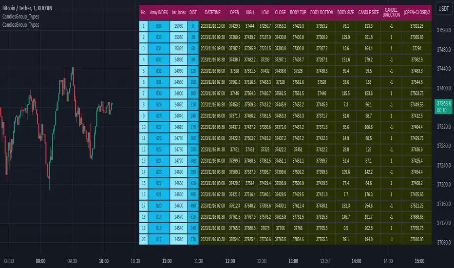
CandlesGroup_TypesLibrary "CandlesGroup_Types"
CandlesGroup Type allows you to efficiently store and access properties of all the candles in your chart.
You can easily manipulate large datasets, work with multiple timeframes, or analyze multiple symbols simultaneously. By encapsulating the properties of each candle within a CandlesGroup object, you gain a convenient and organized way to handle complex candlestick patterns and data.
For usage instructions and detailed examples, please refer to the comments and examples provided in the source code.
method init(_self)
Namespace types: CandlesGroup
Parameters:
_self (CandlesGroup)
method init(_self, propertyNames)
Namespace types: CandlesGroup
Parameters:
_self (CandlesGroup)
propertyNames (string )
method get(_self, key)
get values array from a given property name
Namespace types: CandlesGroup
Parameters:
_self (CandlesGroup) : : CandlesGroup object
key (string) : : key name of selected property. Default is "index"
Returns: values array
method size(_self)
get size of values array. By default it equals to current bar_index
Namespace types: CandlesGroup
Parameters:
_self (CandlesGroup) : : CandlesGroup object
Returns: size of values array
method push(_self, key, value)
push single value to specific property
Namespace types: CandlesGroup
Parameters:
_self (CandlesGroup) : : CandlesGroup object
key (string) : : key name of selected property
value (float) : : property value
Returns: CandlesGroup object
method push(_self, arr)
Namespace types: CandlesGroup
Parameters:
_self (CandlesGroup)
arr (float )
method populate(_self, ohlc)
populate ohlc to CandlesGroup
Namespace types: CandlesGroup
Parameters:
_self (CandlesGroup) : : CandlesGroup object
ohlc (float ) : : array of ohlc
Returns: CandlesGroup object
method populate(_self, values, propertiesNames)
populate values base on given properties Names
Namespace types: CandlesGroup
Parameters:
_self (CandlesGroup) : : CandlesGroup object
values (float ) : : array of property values
propertiesNames (string ) : : an array stores property names. Use as keys to get values
Returns: CandlesGroup object
method populate(_self)
populate values (default setup)
Namespace types: CandlesGroup
Parameters:
_self (CandlesGroup) : : CandlesGroup object
Returns: CandlesGroup object
method lookback(arr, bars_lookback)
get property value on previous candles. For current candle, use *.lookback()
Namespace types: float
Parameters:
arr (float ) : : array of selected property values
bars_lookback (int) : : number of candles lookback. 0 = current candle. Default is 0
Returns: single property value
method highest_within_bars(_self, hiSource, start, end, useIndex)
get the highest property value between specific candles
Namespace types: CandlesGroup
Parameters:
_self (CandlesGroup) : : CandlesGroup object
hiSource (string) : : key name of selected property
start (int) : : start bar for calculation. Default is candles lookback value from current candle. 'index' value is used if 'useIndex' = true
end (int) : : end bar for calculation. Default is candles lookback value from current candle. 'index' value is used if 'useIndex' = true. Default is 0
useIndex (bool) : : use index instead of lookback value. Default = false
Returns: the highest value within candles
method highest_within_bars(_self, returnWithIndex, hiSource, start, end, useIndex)
get the highest property value and bar index between specific candles
Namespace types: CandlesGroup
Parameters:
_self (CandlesGroup) : : CandlesGroup object
returnWithIndex (bool) : : the function only applicable when it is true
hiSource (string) : : key name of selected property
start (int) : : start bar for calculation. Default is candles lookback value from current candle. 'index' value is used if 'useIndex' = true
end (int) : : end bar for calculation. Default is candles lookback value from current candle. 'index' value is used if 'useIndex' = true. Default is 0
useIndex (bool) : : use index instead of lookback value. Default = false
Returns:
method highest_point_within_bars(_self, hiSource, start, end, useIndex)
get a Point object which contains highest property value between specific candles
Namespace types: CandlesGroup
Parameters:
_self (CandlesGroup) : : CandlesGroup object
hiSource (string) : : key name of selected property
start (int) : : start bar for calculation. Default is candles lookback value from current candle. 'index' value is used if 'useIndex' = true
end (int) : : end bar for calculation. Default is candles lookback value from current candle. 'index' value is used if 'useIndex' = true. Default is 0
useIndex (bool) : : use index instead of lookback value. Default = false
Returns: Point object contains highest property value
method lowest_within_bars(_self, loSource, start, end, useIndex)
get the lowest property value between specific candles
Namespace types: CandlesGroup
Parameters:
_self (CandlesGroup) : : CandlesGroup object
loSource (string) : : key name of selected property
start (int) : : start bar for calculation. Default is candles lookback value from current candle. 'index' value is used if 'useIndex' = true
end (int) : : end bar for calculation. Default is candles lookback value from current candle. 'index' value is used if 'useIndex' = true. Default is 0
useIndex (bool) : : use index instead of lookback value. Default = false
Returns: the lowest value within candles
method lowest_within_bars(_self, returnWithIndex, loSource, start, end, useIndex)
get the lowest property value and bar index between specific candles
Namespace types: CandlesGroup
Parameters:
_self (CandlesGroup) : : CandlesGroup object
returnWithIndex (bool) : : the function only applicable when it is true
loSource (string) : : key name of selected property
start (int) : : start bar for calculation. Default is candles lookback value from current candle. 'index' value is used if 'useIndex' = true
end (int) : : end bar for calculation. Default is candles lookback value from current candle. 'index' value is used if 'useIndex' = true. Default is 0
useIndex (bool) : : use index instead of lookback value. Default = false
Returns:
method lowest_point_within_bars(_self, loSource, start, end, useIndex)
get a Point object which contains lowest property value between specific candles
Namespace types: CandlesGroup
Parameters:
_self (CandlesGroup) : : CandlesGroup object
loSource (string) : : key name of selected property
start (int) : : start bar for calculation. Default is candles lookback value from current candle. 'index' value is used if 'useIndex' = true
end (int) : : end bar for calculation. Default is candles lookback value from current candle. 'index' value is used if 'useIndex' = true. Default is 0
useIndex (bool) : : use index instead of lookback value. Default = false
Returns: Point object contains lowest property value
method time2bar(_self, t)
Convert UNIX time to bar index of active chart
Namespace types: CandlesGroup
Parameters:
_self (CandlesGroup) : : CandlesGroup object
t (int) : : UNIX time
Returns: bar index
method time2bar(_self, timezone, YYYY, MMM, DD, hh, mm, ss)
Convert timestamp to bar index of active chart. User defined timezone required
Namespace types: CandlesGroup
Parameters:
_self (CandlesGroup) : : CandlesGroup object
timezone (string) : : User defined timezone
YYYY (int) : : Year
MMM (int) : : Month
DD (int) : : Day
hh (int) : : Hour. Default is 0
mm (int) : : Minute. Default is 0
ss (int) : : Second. Default is 0
Returns: bar index
method time2bar(_self, YYYY, MMM, DD, hh, mm, ss)
Convert timestamp to bar index of active chart
Namespace types: CandlesGroup
Parameters:
_self (CandlesGroup) : : CandlesGroup object
YYYY (int) : : Year
MMM (int) : : Month
DD (int) : : Day
hh (int) : : Hour. Default is 0
mm (int) : : Minute. Default is 0
ss (int) : : Second. Default is 0
Returns: bar index
method get_prop_from_time(_self, key, t)
get single property value from UNIX time
Namespace types: CandlesGroup
Parameters:
_self (CandlesGroup) : : CandlesGroup object
key (string) : : key name of selected property
t (int) : : UNIX time
Returns: single property value
method get_prop_from_time(_self, key, timezone, YYYY, MMM, DD, hh, mm, ss)
get single property value from timestamp. User defined timezone required
Namespace types: CandlesGroup
Parameters:
_self (CandlesGroup) : : CandlesGroup object
key (string) : : key name of selected property
timezone (string) : : User defined timezone
YYYY (int) : : Year
MMM (int) : : Month
DD (int) : : Day
hh (int) : : Hour. Default is 0
mm (int) : : Minute. Default is 0
ss (int) : : Second. Default is 0
Returns: single property value
method get_prop_from_time(_self, key, YYYY, MMM, DD, hh, mm, ss)
get single property value from timestamp
Namespace types: CandlesGroup
Parameters:
_self (CandlesGroup) : : CandlesGroup object
key (string) : : key name of selected property
YYYY (int) : : Year
MMM (int) : : Month
DD (int) : : Day
hh (int) : : Hour. Default is 0
mm (int) : : Minute. Default is 0
ss (int) : : Second. Default is 0
Returns: single property value
method bar2time(_self, index)
Convert bar index of active chart to UNIX time
Namespace types: CandlesGroup
Parameters:
_self (CandlesGroup) : : CandlesGroup object
index (int) : : bar index
Returns: UNIX time
Point
A point on chart
Fields:
price (series float) : : price value
bar (series int) : : bar index
bartime (series int) : : time in UNIX format of bar
Property
Property object which contains values of all candles
Fields:
name (series string) : : name of property
values (float ) : : an array stores values of all candles. Size of array = bar_index
CandlesGroup
Candles Group object which contains properties of all candles
Fields:
propertyNames (string ) : : an array stores property names. Use as keys to get values
properties (Property ) : : array of Property objects
SILLibrary "SIL"
mean_src(x, y)
calculates moving average : x is the source of price (OHLC) & y = the lookback period
Parameters:
x
y
stan_dev(x, y, z)
calculates standard deviation, x = source of price (OHLC), y = the average lookback, z = average given prior two float and intger inputs, call the f_avg_src() function in f_stan_dev()
Parameters:
x
y
z
vawma(x, y)
calculates volume weighted moving average, x = source of price (OHLC), y = loookback period
Parameters:
x
y
gethurst(x, y, z)
calculates the Hurst Exponent and Hurst Exponent average, x = source of price (OHLC), y = lookback period for Hurst Exponent Calculation, z = lookback period for average Hurst Exponent
Parameters:
x
y
z

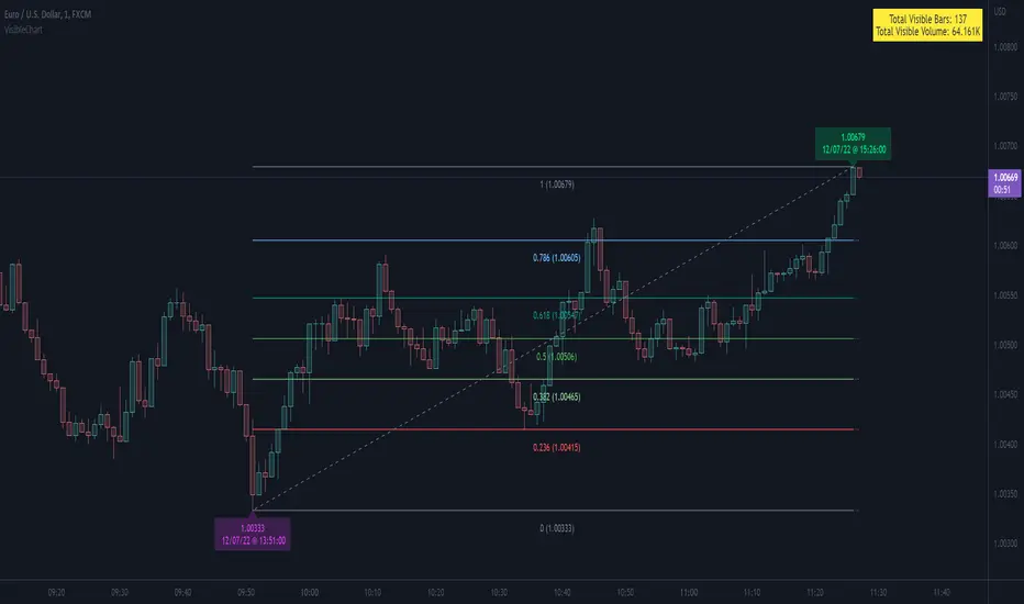
VisibleChart█ OVERVIEW
This library is a Pine programmer’s tool containing functions that return values calculated from the range of visible bars on the chart.
This is now possible in Pine Script™ thanks to the recently-released chart.left_visible_bar_time and chart.right_visible_bar_time built-ins, which return the opening time of the leftmost and rightmost bars on the chart. These values update as traders scroll or zoom their charts, which gives way to a class of indicators that can dynamically recalculate and draw visuals on visible bars only, as users scroll or zoom their charts. We hope this library's functions help you make the most of the world of possibilities these new built-ins provide for Pine scripts.
For an example of a script using this library, have a look at the Chart VWAP indicator.
█ CONCEPTS
Chart properties
The new chart.left_visible_bar_time and chart.right_visible_bar_time variables return the opening time of the leftmost and rightmost bars on the chart. They are only two of many new built-ins in the `chart.*` namespace. See this blog post for more information, or look them up by typing "chart." in the Pine Script™ Reference Manual .
Dynamic recalculation of scripts on visible bars
Any script using chart.left_visible_bar_time or chart.right_visible_bar_time acquires a unique property, which triggers its recalculation when traders scroll or zoom their charts in such a way that the range of visible bars on the chart changes. This library's functions use the two recent built-ins to derive various values from the range of visible bars.
Designing your scripts for dynamic recalculation
For the library's functions to work correctly, they must be called on every bar. For reliable results, assign their results to global variables and then use the variables locally where needed — not the raw function calls.
Some functions like `barIsVisible()` or `open()` will return a value starting on the leftmost visible bar. Others such as `high()` or `low()` will also return a value starting on the leftmost visible bar, but their correct value can only be known on the rightmost visible bar, after all visible bars have been analyzed by the script.
You can plot values as the script executes on visible bars, but efficient code will, when possible, create resource-intensive labels, lines or tables only once in the global scope using var , and then use the setter functions to modify their properties on the last bar only. The example code included in this library uses this method.
Keep in mind that when your script uses chart.left_visible_bar_time or chart.right_visible_bar_time , your script will recalculate on all bars each time the user scrolls or zooms their chart. To provide script users with the best experience you should strive to keep calculations to a minimum and use efficient code so that traders are not always waiting for your script to recalculate every time they scroll or zoom their chart.
Another aspect to consider is the fact that the rightmost visible bar will not always be the last bar in the dataset. When script users scroll back in time, a large portion of the time series the script calculates on may be situated after the rightmost visible bar. We can never assume the rightmost visible bar is also the last bar of the time series. Use `barIsVisible()` to restrict calculations to visible bars, but also consider that your script can continue to execute past them.
Look first. Then leap.
█ FUNCTIONS
The library contains the following functions:
barIsVisible()
Condition to determine if a given bar is within the users visible time range.
Returns: (bool) True if the the calling bar is between the `chart.left_visible_bar_time` and the `chart.right_visible_bar_time`.
high()
Determines the value of the highest `high` in visible bars.
Returns: (float) The maximum high value of visible chart bars.
highBarIndex()
Determines the `bar_index` of the highest `high` in visible bars.
Returns: (int) The `bar_index` of the `high()`.
highBarTime()
Determines the bar time of the highest `high` in visible bars.
Returns: (int) The `time` of the `high()`.
low()
Determines the value of the lowest `low` in visible bars.
Returns: (float) The minimum low value of visible chart bars.
lowBarIndex()
Determines the `bar_index` of the lowest `low` in visible bars.
Returns: (int) The `bar_index` of the `low()`.
lowBarTime()
Determines the bar time of the lowest `low` in visible bars.
Returns: (int) The `time` of the `low()`.
open()
Determines the value of the opening price in the visible chart time range.
Returns: (float) The `open` of the leftmost visible chart bar.
close()
Determines the value of the closing price in the visible chart time range.
Returns: (float) The `close` of the rightmost visible chart bar.
leftBarIndex()
Determines the `bar_index` of the leftmost visible chart bar.
Returns: (int) A `bar_index`.
rightBarIndex()
Determines the `bar_index` of the rightmost visible chart bar.
Returns: (int) A `bar_index`
bars()
Determines the number of visible chart bars.
Returns: (int) The number of bars.
volume()
Determines the sum of volume of all visible chart bars.
Returns: (float) The cumulative sum of volume.
ohlcv()
Determines the open, high, low, close, and volume sum of the visible bar time range.
Returns: ( ) A tuple of the OHLCV values for the visible chart bars. Example: open is chart left, high is the highest visible high, etc.
chartYPct(pct)
Determines a price level as a percentage of the visible bar price range, which depends on the chart's top/bottom margins in "Settings/Appearance".
Parameters:
pct : (series float) Percentage of the visible price range (50 is 50%). Negative values are allowed.
Returns: (float) A price level equal to the `pct` of the price range between the high and low of visible chart bars. Example: 50 is halfway between the visible high and low.
chartXTimePct(pct)
Determines a time as a percentage of the visible bar time range.
Parameters:
pct : (series float) Percentage of the visible time range (50 is 50%). Negative values are allowed.
Returns: (float) A time in UNIX format equal to the `pct` of the time range from the `chart.left_visible_bar_time` to the `chart.right_visible_bar_time`. Example: 50 is halfway from the leftmost visible bar to the rightmost.
chartXIndexPct(pct)
Determines a `bar_index` as a percentage of the visible bar time range.
Parameters:
pct : (series float) Percentage of the visible time range (50 is 50%). Negative values are allowed.
Returns: (float) A time in UNIX format equal to the `pct` of the time range from the `chart.left_visible_bar_time` to the `chart.right_visible_bar_time`. Example: 50 is halfway from the leftmost visible bar to the rightmost.
whenVisible(src, whenCond, length)
Creates an array containing the `length` last `src` values where `whenCond` is true for visible chart bars.
Parameters:
src : (series int/float) The source of the values to be included.
whenCond : (series bool) The condition determining which values are included. Optional. The default is `true`.
length : (simple int) The number of last values to return. Optional. The default is all values.
Returns: (float ) The array ID of the accumulated `src` values.
avg(src)
Gathers values of the source over visible chart bars and averages them.
Parameters:
src : (series int/float) The source of the values to be averaged. Optional. Default is `close`.
Returns: (float) A cumulative average of values for the visible time range.
median(src)
Calculates the median of a source over visible chart bars.
Parameters:
src : (series int/float) The source of the values. Optional. Default is `close`.
Returns: (float) The median of the `src` for the visible time range.
vVwap(src)
Calculates a volume-weighted average for visible chart bars.
Parameters:
src : (series int/float) Source used for the VWAP calculation. Optional. Default is `hlc3`.
Returns: (float) The VWAP for the visible time range.
How to avoid repainting when using security() - PineCoders FAQNOTE
The non-repainting technique in this publication that relies on bar states is now deprecated, as we have identified inconsistencies that undermine its credibility as a universal solution. The outputs that use the technique are still available for reference in this publication. However, we do not endorse its usage. See this publication for more information about the current best practices for requesting HTF data and why they work.
This indicator shows how to avoid repainting when using the security() function to retrieve information from higher timeframes.
What do we mean by repainting?
Repainting is used to describe three different things, in what we’ve seen in TV members comments on indicators:
1. An indicator showing results that change during the realtime bar, whether the script is using the security() function or not, e.g., a Buy signal that goes on and then off, or a plot that changes values.
2. An indicator that uses future data not yet available on historical bars.
3. An indicator that uses a negative offset= parameter when plotting in order to plot information on past bars.
The repainting types we will be discussing here are the first two types, as the third one is intentional—sometimes even intentionally misleading when unscrupulous script writers want their strategy to look better than it is.
Let’s be clear about one thing: repainting is not caused by a bug ; it is caused by the different context between historical bars and the realtime bar, and script coders or users not taking the necessary precautions to prevent it.
Why should repainting be avoided?
Repainting matters because it affects the behavior of Pine scripts in the realtime bar, where the action happens and counts, because that is when traders (or our systems) take decisions where odds must be in our favor.
Repainting also matters because if you test a strategy on historical bars using only OHLC values, and then run that same code on the realtime bar with more than OHLC information, scripts not properly written or misconfigured alerts will alter the strategy’s behavior. At that point, you will not be running the same strategy you tested, and this invalidates your test results , which were run while not having the additional price information that is available in the realtime bar.
The realtime bar on your charts is only one bar, but it is a very important bar. Coding proper strategies and indicators on TV requires that you understand the variations in script behavior and how information available to the script varies between when the script is running on historical and realtime bars.
How does repainting occur?
Repainting happens because of something all traders instinctively crave: more information. Contrary to trader lure, more information is not always better. In the realtime bar, all TV indicators (a.k.a. studies ) execute every time price changes (i.e. every tick ). TV strategies will also behave the same way if they use the calc_on_every_tick = true parameter in their strategy() declaration statement (the parameter’s default value is false ). Pine coders must decide if they want their code to use the realtime price information as it comes in, or wait for the realtime bar to close before using the same OHLC values for that bar that would be used on historical bars.
Strategy modelers often assume that using realtime price information as it comes in the realtime bar will always improve their results. This is incorrect. More information does not necessarily improve performance because it almost always entails more noise. The extra information may or may not improve results; one cannot know until the code is run in realtime for enough time to provide data that can be analyzed and from which somewhat reliable conclusions can be derived. In any case, as was stated before, it is critical to understand that if your strategy is taking decisions on realtime tick data, you are NOT running the same strategy you tested on historical bars with OHLC values only.
How do we avoid repainting?
It comes down to using reliable information and properly configuring alerts, if you use them. Here are the main considerations:
1. If your code is using security() calls, use the syntax we propose to obtain reliable data from higher timeframes.
2. If your script is a strategy, do not use the calc_on_every_tick = true parameter unless your strategy uses previous bar information to calculate.
3. If your script is a study and is using current timeframe information that is compared to values obtained from a higher timeframe, even if you can rely on reliable higher timeframe information because you are correctly using the security() function, you still need to ensure the realtime bar’s information you use (a cross of current close over a higher timeframe MA, for example) is consistent with your backtest methodology, i.e. that your script calculates on the close of the realtime bar. If your system is using alerts, the simplest solution is to configure alerts to trigger Once Per Bar Close . If you are not using alerts, the best solution is to use information from the preceding bar. When using previous bar information, alerts can be configured to trigger Once Per Bar safely.
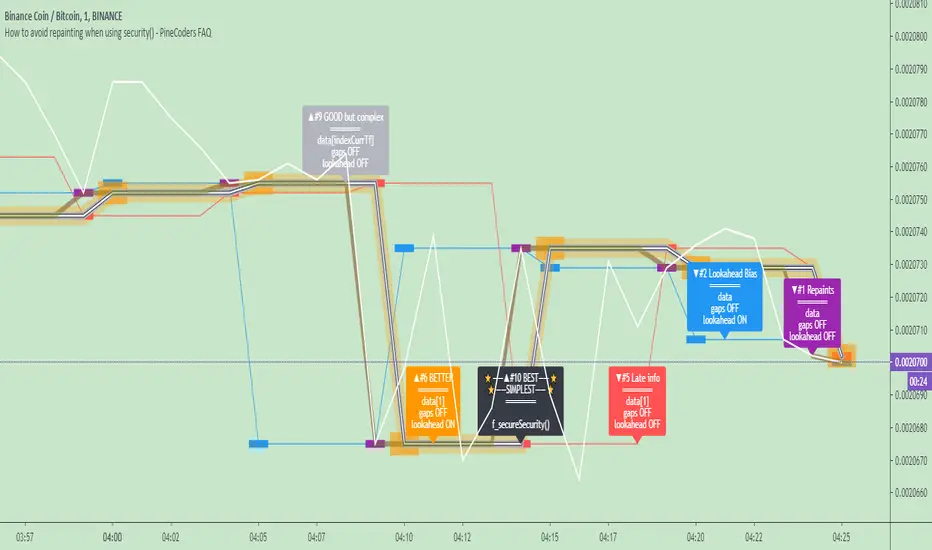
What does this indicator do?
It shows results for 9 different ways of using the security() function and illustrates the simplest and most effective way to avoid repainting, i.e. using security() as in the example above. To show the indicator’s lines the most clearly, price on the chart is shown with a black line rather than candlesticks. This indicator also shows how misusing security() produces repainting. All combinations of using a 0 or 1 offset to reference the series used in the security() , as well as all combinations of values for the gaps= and lookahead= parameters are shown.
The close in the call labeled “BEST” means that once security has reached the upper timeframe (1 day in our case), it will fetch the previous day’s value.
The gaps= parameter is not specified as it is off by default and that is what we need. This ensures that the value returned by security() will not contain na values on any of our chart’s bars.
The lookahead security() to use the last available value for the higher timeframe bar we are using (the previous day, in our case). This ensures that security() will return the value at the end of the higher timeframe, even if it has not occurred yet. In our case, this has no negative impact since we are requesting the previous day’s value, with has already closed.
The indicator’s Settings/Inputs allow you to set:
- The higher timeframe security() calls will use
- The source security() calls will use
- If you want identifying labels printed on the lines that have no gaps (the lines containing gaps are plotted using very thick lines that appear as horizontal blocks of one bar in length)
For the lines to be plotted, you need to be on a smaller timeframe than the one used for the security() calls.
Comments in the code explain what’s going on.
Look first. Then leap.
Probability Cone█ Overview:
Probability Cone is based on the Expected Move . While Expected Move only shows the historical value band on every bar, probability panel extend the period in the future and plot a cone or curve shape of the probable range. It plots the range from bar 1 all the way to bar 31.
In this model, we assume asset price follows a log-normal distribution and the log return follows a normal distribution.
Note: Normal distribution is just an assumption; it's not the real distribution of return.
The area of probability range is based on an inverse normal cumulative distribution function. The inverse cumulative distribution gives the range of price for given input probability. People can adjust the range by adjusting the standard deviation in the settings. The probability of the entered standard deviation will be shown at the edges of the probability cone.
The shown 68% and 95% probabilities correspond to the full range between the two blue lines of the cone (68%) and the two purple lines of the cone (95%). The probabilities suggest the % of outcomes or data that are expected to lie within this range. It does not suggest the probability of reaching those price levels.
Note: All these probabilities are based on the normal distribution assumption for returns. It's the estimated probability, not the actual probability.
█ Volatility Models :
Sample SD : traditional sample standard deviation, most commonly used, use (n-1) period to adjust the bias
Parkinson : Uses High/ Low to estimate volatility, assumes continuous no gap, zero mean no drift, 5 times more efficient than Close to Close
Garman Klass : Uses OHLC volatility, zero drift, no jumps, about 7 times more efficient
Yangzhang Garman Klass Extension : Added jump calculation in Garman Klass, has the same value as Garman Klass on markets with no gaps.
about 8 x efficient
Rogers : Uses OHLC, Assume non-zero mean volatility, handles drift, does not handle jump 8 x efficient.
EWMA : Exponentially Weighted Volatility. Weight recently volatility more, more reactive volatility better in taking account of volatility autocorrelation and cluster.
YangZhang : Uses OHLC, combines Rogers and Garmand Klass, handles both drift and jump, 14 times efficient, alpha is the constant to weight rogers volatility to minimize variance.
Median absolute deviation : It's a more direct way of measuring volatility. It measures volatility without using Standard deviation. The MAD used here is adjusted to be an unbiased estimator.
You can learn more about each of the volatility models in out Historical Volatility Estimators indicator.
█ How to use
Volatility Period is the sample size for variance estimation. A longer period makes the estimation range more stable less reactive to recent price. Distribution is more significant on larger sample size. A short period makes the range more responsive to recent price. Might be better for high volatility clusters.
People usually assume the mean of returns to be zero. To be more accurate, we can consider the drift in price from calculating the geometric mean of returns. Drift happens in the long run, so short lookback periods are not recommended.
The shape of the cone will be skewed and have a directional bias when the length of mean is short. It might be more adaptive to the current price or trend, but more accurate estimation should use a longer period for the mean.
Using a short look back for mean will make the cone having a directional bias.
When we are estimating the future range for time > 1, we typically assume constant volatility and the returns to be independent and identically distributed. We scale the volatility in term of time to get future range. However, when there's autocorrelation in returns( when returns are not independent), the assumption fails to take account of this effect. Volatility scaled with autocorrelation is required when returns are not iid. We use an AR(1) model to scale the first-order autocorrelation to adjust the effect. Returns typically don't have significant autocorrelation. Adjustment for autocorrelation is not usually needed. A long length is recommended in Autocorrelation calculation.
Note: The significance of autocorrelation can be checked on an ACF indicator.
ACF
Time back settings shift the estimation period back by the input number. It's the origin of when the probability cone start to estimation it's range.
E.g., When time back = 5, the probability cone start its prediction interval estimation from 5 bars ago. So for time back = 5 , it estimates the probability range from 5 bars ago to X number of bars in the future, specified by the Forecast Period (max 1000).
█ Warnings:
People should not blindly trust the probability. They should be aware of the risk evolves by using the normal distribution assumption. The real return has skewness and high kurtosis. While skewness is not very significant, the high kurtosis should be noticed. The Real returns have much fatter tails than the normal distribution, which also makes the peak higher. This property makes the tail ranges such as range more than 2SD highly underestimate the actual range and the body such as 1 SD slightly overestimate the actual range. For ranges more than 2SD, people shouldn't trust them. They should beware of extreme events in the tails.
The uncertainty in future bars makes the range wider. The overestimate effect of the body is partly neutralized when it's extended to future bars. We encourage people who use this indicator to further investigate the Historical Volatility Estimators , Fast Autocorrelation Estimator , Expected Move and especially the Linear Moments Indicator .
The probability is only for the closing price, not wicks. It only estimates the probability of the price closing at this level, not in between.

Expected Move BandsExpected move is the amount that an asset is predicted to increase or decrease from its current price, based on the current levels of volatility.
In this model, we assume asset price follows a log-normal distribution and the log return follows a normal distribution.
Note: Normal distribution is just an assumption, it's not the real distribution of return
Settings:
"Estimation Period Selection" is for selecting the period we want to construct the prediction interval.
For "Current Bar", the interval is calculated based on the data of the previous bar close. Therefore changes in the current price will have little effect on the range. What current bar means is that the estimated range is for when this bar close. E.g., If the Timeframe on 4 hours and 1 hour has passed, the interval is for how much time this bar has left, in this case, 3 hours.
For "Future Bars", the interval is calculated based on the current close. Therefore the range will be very much affected by the change in the current price. If the current price moves up, the range will also move up, vice versa. Future Bars is estimating the range for the period at least one bar ahead.
There are also other source selections based on high low.
Time setting is used when "Future Bars" is chosen for the period. The value in time means how many bars ahead of the current bar the range is estimating. When time = 1, it means the interval is constructing for 1 bar head. E.g., If the timeframe is on 4 hours, then it's estimating the next 4 hours range no matter how much time has passed in the current bar.
Note: It's probably better to use "probability cone" for visual presentation when time > 1
Volatility Models :
Sample SD: traditional sample standard deviation, most commonly used, use (n-1) period to adjust the bias
Parkinson: Uses High/ Low to estimate volatility, assumes continuous no gap, zero mean no drift, 5 times more efficient than Close to Close
Garman Klass: Uses OHLC volatility, zero drift, no jumps, about 7 times more efficient
Yangzhang Garman Klass Extension: Added jump calculation in Garman Klass, has the same value as Garman Klass on markets with no gaps.
about 8 x efficient
Rogers: Uses OHLC, Assume non-zero mean volatility, handles drift, does not handle jump 8 x efficient
EWMA: Exponentially Weighted Volatility. Weight recently volatility more, more reactive volatility better in taking account of volatility autocorrelation and cluster.
YangZhang: Uses OHLC, combines Rogers and Garmand Klass, handles both drift and jump, 14 times efficient, alpha is the constant to weight rogers volatility to minimize variance.
Median absolute deviation: It's a more direct way of measuring volatility. It measures volatility without using Standard deviation. The MAD used here is adjusted to be an unbiased estimator.
Volatility Period is the sample size for variance estimation. A longer period makes the estimation range more stable less reactive to recent price. Distribution is more significant on a larger sample size. A short period makes the range more responsive to recent price. Might be better for high volatility clusters.
Standard deviations:
Standard Deviation One shows the estimated range where the closing price will be about 68% of the time.
Standard Deviation two shows the estimated range where the closing price will be about 95% of the time.
Standard Deviation three shows the estimated range where the closing price will be about 99.7% of the time.
Note: All these probabilities are based on the normal distribution assumption for returns. It's the estimated probability, not the actual probability.
Manually Entered Standard Deviation shows the range of any entered standard deviation. The probability of that range will be presented on the panel.
People usually assume the mean of returns to be zero. To be more accurate, we can consider the drift in price from calculating the geometric mean of returns. Drift happens in the long run, so short lookback periods are not recommended. Assuming zero mean is recommended when time is not greater than 1.
When we are estimating the future range for time > 1, we typically assume constant volatility and the returns to be independent and identically distributed. We scale the volatility in term of time to get future range. However, when there's autocorrelation in returns( when returns are not independent), the assumption fails to take account of this effect. Volatility scaled with autocorrelation is required when returns are not iid. We use an AR(1) model to scale the first-order autocorrelation to adjust the effect. Returns typically don't have significant autocorrelation. Adjustment for autocorrelation is not usually needed. A long length is recommended in Autocorrelation calculation.
Note: The significance of autocorrelation can be checked on an ACF indicator.
ACF
The multimeframe option enables people to use higher period expected move on the lower time frame. People should only use time frame higher than the current time frame for the input. An error warning will appear when input Tf is lower. The input format is multiplier * time unit. E.g. : 1D
Unit: M for months, W for Weeks, D for Days, integers with no unit for minutes (E.g. 240 = 240 minutes). S for Seconds.
Smoothing option is using a filter to smooth out the range. The filter used here is John Ehler's supersmoother. It's an advance smoothing technique that gets rid of aliasing noise. It affects is similar to a simple moving average with half the lookback length but smoother and has less lag.
Note: The range here after smooth no long represent the probability
Panel positions can be adjusted in the settings.
X position adjusts the horizontal position of the panel. Higher X moves panel to the right and lower X moves panel to the left.
Y position adjusts the vertical position of the panel. Higher Y moves panel up and lower Y moves panel down.
Step line display changes the style of the bands from line to step line. Step line is recommended because it gets rid of the directional bias of slope of expected move when displaying the bands.
Warnings:
People should not blindly trust the probability. They should be aware of the risk evolves by using the normal distribution assumption. The real return has skewness and high kurtosis. While skewness is not very significant, the high kurtosis should be noticed. The Real returns have much fatter tails than the normal distribution, which also makes the peak higher. This property makes the tail ranges such as range more than 2SD highly underestimate the actual range and the body such as 1 SD slightly overestimate the actual range. For ranges more than 2SD, people shouldn't trust them. They should beware of extreme events in the tails.
Different volatility models provide different properties if people are interested in the accuracy and the fit of expected move, they can try expected move occurrence indicator. (The result also demonstrate the previous point about the drawback of using normal distribution assumption).
Expected move Occurrence Test
The prediction interval is only for the closing price, not wicks. It only estimates the probability of the price closing at this level, not in between. E.g., If 1 SD range is 100 - 200, the price can go to 80 or 230 intrabar, but if the bar close within 100 - 200 in the end. It's still considered a 68% one standard deviation move.

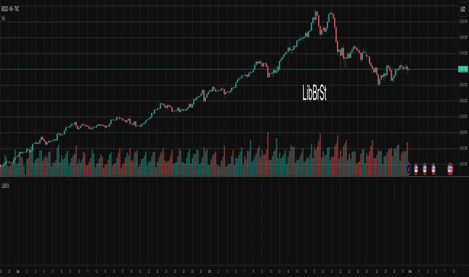
LibBrStLibrary "LibBrSt"
This is a library for quantitative analysis, designed to estimate
the statistical properties of price movements *within* a single
OHLC bar, without requiring access to tick data. It provides a
suite of estimators based on various statistical and econometric
models, allowing for analysis of intra-bar volatility and
price distribution.
Key Capabilities:
1. **Price Distribution Models (`PriceEst`):** Provides a selection
of estimators that model intra-bar price action as a probability
distribution over the range. This allows for the
calculation of the intra-bar mean (`priceMean`) and standard
deviation (`priceStdDev`) in absolute price units. Models include:
- **Symmetric Models:** `uniform`, `triangular`, `arcsine`,
`betaSym`, and `t4Sym` (Student-t with fat tails).
- **Skewed Models:** `betaSkew` and `t4Skew`, which adjust
their shape based on the Open/Close position.
- **Model Assumptions:** The skewed models rely on specific
internal constants. `betaSkew` uses a fixed concentration
parameter (`BETA_SKEW_CONCENTRATION = 4.0`), and `t4Sym`/`t4Skew`
use a heuristic scaling factor (`T4_SHAPE_FACTOR`)
to map the distribution.
2. **Econometric Log-Return Estimators (`LogEst`):** Includes a set of
econometric estimators for calculating the volatility (`logStdDev`)
and drift (`logMean`) of logarithmic returns within a single bar.
These are unit-less measures. Models include:
- **Parkinson (1980):** A High-Low range estimator.
- **Garman-Klass (1980):** An OHLC-based estimator.
- **Rogers-Satchell (1991):** An OHLC estimator that accounts
for non-zero drift.
3. **Distribution Analysis (PDF/CDF):** Provides functions to work
with the Probability Density Function (`pricePdf`) and
Cumulative Distribution Function (`priceCdf`) of the
chosen price model.
- **Note on `priceCdf`:** This function uses analytical (exact)
calculations for the `uniform`, `triangular`, and `arcsine`
models. For all other models (e.g., `betaSkew`, `t4Skew`),
it uses **numerical integration (Simpson's rule)** as
an approximation of the cumulative probability.
4. **Mathematical Functions:** The library's Beta distribution
models (`betaSym`, `betaSkew`) are supported by an internal
implementation of the natural log-gamma function, which is
based on the Lanczos approximation.
---
**DISCLAIMER**
This library is provided "AS IS" and for informational and
educational purposes only. It does not constitute financial,
investment, or trading advice.
The author assumes no liability for any errors, inaccuracies,
or omissions in the code. Using this library to build
trading indicators or strategies is entirely at your own risk.
As a developer using this library, you are solely responsible
for the rigorous testing, validation, and performance of any
scripts you create based on these functions. The author shall
not be held liable for any financial losses incurred directly
or indirectly from the use of this library or any scripts
derived from it.
priceStdDev(estimator, offset)
Estimates **σ̂** (standard deviation) *in price units* for the current
bar, according to the chosen `PriceEst` distribution assumption.
Parameters:
estimator (series PriceEst) : series PriceEst Distribution assumption (see enum).
offset (int) : series int To offset the calculated bar
Returns: series float σ̂ ≥ 0 ; `na` if undefined (e.g. zero range).
priceMean(estimator, offset)
Estimates **μ̂** (mean price) for the chosen `PriceEst` within the
current bar.
Parameters:
estimator (series PriceEst) : series PriceEst Distribution assumption (see enum).
offset (int) : series int To offset the calculated bar
Returns: series float μ̂ in price units.
pricePdf(estimator, price, offset)
Probability-density under the chosen `PriceEst` model.
**Returns 0** when `p` is outside the current bar’s .
Parameters:
estimator (series PriceEst) : series PriceEst Distribution assumption (see enum).
price (float) : series float Price level to evaluate.
offset (int) : series int To offset the calculated bar
Returns: series float Density value.
priceCdf(estimator, upper, lower, steps, offset)
Cumulative probability **between** `upper` and `lower` under
the chosen `PriceEst` model. Outside-bar regions contribute zero.
Uses a fast, analytical calculation for Uniform, Triangular, and
Arcsine distributions, and defaults to numerical integration
(Simpson's rule) for more complex models.
Parameters:
estimator (series PriceEst) : series PriceEst Distribution assumption (see enum).
upper (float) : series float Upper Integration Boundary.
lower (float) : series float Lower Integration Boundary.
steps (int) : series int # of sub-intervals for numerical integration (if used).
offset (int) : series int To offset the calculated bar.
Returns: series float Probability mass ∈ .
logStdDev(estimator, offset)
Estimates **σ̂** (standard deviation) of *log-returns* for the current bar.
Parameters:
estimator (series LogEst) : series LogEst Distribution assumption (see enum).
offset (int) : series int To offset the calculated bar
Returns: series float σ̂ (unit-less); `na` if undefined.
logMean(estimator, offset)
Estimates μ̂ (mean log-return / drift) for the chosen `LogEst`.
The returned value is consistent with the assumptions of the
selected volatility estimator.
Parameters:
estimator (series LogEst) : series LogEst Distribution assumption (see enum).
offset (int) : series int To offset the calculated bar
Returns: series float μ̂ (unit-less log-return).
HTF Live View - GSK-VIZAG-AP-INDIA📘 HTF Live View — GSK-VIZAG-AP-INDIA
🧩 Overview
The HTF Live View indicator provides a real-time visual representation of higher-timeframe (HTF) candle structures — such as 15min, 30min, 1H, 4H, and Daily — all derived directly from live 1-minute data.
This allows traders to see how higher timeframe candles are forming within the current session — without switching chart timeframes.
⚙️ Core Features
📊 Live Multi-Timeframe OHLC Tracking
Continuously calculates and displays Open, High, Low, and Close values for each key timeframe (15m, 30m, 1H, 4H, and Daily) based on the ongoing session.
⏱ Session-Aware Calculation
Automatically syncs with market hours defined by user-selected start and end times. Works across multiple timezones for global compatibility.
🕹 Visual Candle Representation
Draws mini-candles on the chart for each higher timeframe to represent their current body and wick — updated live.
Green body → bullish development
Red body → bearish development
📅 Informative Table Panel
Displays a summary table showing:
Timeframe label
Period (start–end time)
Live OHLC values
Color-coded close values
🌍 Timezone Support
Fully compatible with common regions such as Asia/Kolkata, New York, London, Tokyo, and Sydney.
🔧 User Inputs
Parameter Description
Market Start Hour/Minute Define session start time (default: 09:15)
Session End Hour/Minute Define market close (default: 15:30)
Timezone Select your preferred timezone for session alignment
💡 How It Works
The indicator uses a rolling OHLC calculation function that dynamically computes candle values based on elapsed session time.
Each timeframe (15m, 30m, 1H, 4H, and Daily) is built from 1-minute data to maintain precision even during intraday updates.
Both a visual representation (candles and wicks) and a data table (numeric summary) are displayed for clarity.
🧠 Use Cases
Monitor how HTF candles are forming live without switching chart intervals.
Understand intraday structure shifts (e.g., when 1H turns from red to green).
Confirm trend alignment across multiple timeframes visually.
Combine with your volume, delta, or liquidity tools for deeper confluence.
🪶 Signature
Developed by GSK-VIZAG-AP-INDIA
© prowelltraders — Educational and analytical use only.
⚠️ Disclaimer
This indicator is for educational and informational purposes only.
It does not provide financial advice or guaranteed trading results.
Always perform your own analysis before making investment decisions.

Time LevelsTime Levels is a customizable TradingView indicator designed to mark critical intraday price levels based on specific time inputs. This tool helps traders identify significant Open/High/Low/Close (OHLC) levels, support & resistance (S&R) zones, and potential Judas Swing manipulation points—aligned with selected timeframes and adjusted to any time zone via UTC offset.
🔧 Key Features:
OHLC/OLHC Levels: Automatically draws horizontal lines at the candle’s open price for up to four specified time points. Ideal for marking session opens, closes, or key intraday levels.
Support & Resistance Zones: Highlights two time-based S&R levels that can help identify discount and premium pricing zones.
Judas Swing Detection: Marks potential liquidity grab zones (Judas Swings) at three user-defined times, assisting in identifying manipulation and smart money entry points.
Global Timezone Support: Includes a UTC offset input to align levels accurately with your trading session, regardless of your location.
Full Customization: Personalize the color, style (solid, dashed, dotted), and thickness of each line independently for OHLC, S&R, and Judas levels.
🛠️ Use Cases:
New York / London open price tracking
ICT-based SMC level marking
Predefined time-based liquidity level visualizations
Institutional-level price reactions (e.g., during specific market opens)
This indicator is best suited for intraday and short-term (especially ICT) traders looking to bring precision and consistency into their technical analysis framework.

LineReg Candles with Hma filterOverview
Purpose:
The indicator creates “LinReg Candles” by recalculating OHLC values using linear regression (to smooth out noise) and overlays additional features such as a customizable signal line and an HMA (Hull Moving Average) filter for trend detection. It also plots buy/sell signals and supports alerts.
Customization:
Users can adjust settings for signal smoothing (choosing SMA, EMA, or WMA), HMA periods (preset for Scalping/Intraday or custom values), linear regression length, colors, display options, and alert messages. Inputs are organized into groups for clarity.
Input Definitions
Signal Settings:
signal_length and smoothingType define the period and method used to smooth the close price, creating a signal line.
HMA Filter Settings:
A dropdown (t_type) lets you choose between Scalping, Intraday, or Custom. Based on this, three HMA periods (hma1, hma2, hma3) are set either to fixed values or user-defined custom inputs.
LinReg Settings:
Users can toggle linear regression for OHLC values (lin_reg) and set its period (linreg_length) to reduce price noise.
Color and Display Settings:
These control the colors for buy/sell candles, default bullish/bearish candles, markers, and background highlighting. Display toggles decide whether to show the background, signal line, HMA filter, and the recalculated candles.
Alert and Plot Customization:
Alerts can be enabled with custom messages. Additionally, line width and transparency for the plotted signal and HMA lines are adjustable.
Function Definitions
calcOHLC Function:
Computes OHLC values using linear regression if enabled. Otherwise, it returns the raw price values. This helps in reducing noise.
calcSignalLine Function:
Applies the chosen moving average (SMA, EMA, or WMA) to smooth the recalculated close values and generate a signal line.
getBaseCandleColor Function:
Determines the candle’s base color. It assigns buy/sell colors if specific crossover conditions are met; if not, it defaults to bullish (green) or bearish (red) based on the open/close relationship.
HMA Filter Calculations
HMA Computation:
The script calculates three HMAs (ma1, ma2, ma3) for different periods.
Trend Determination:
It sets a bullish condition (bcn) when ma3 is lower than both ma1 and ma2 with ma1 above ma2. Conversely, a bearish condition (scn) is set when ma3 is higher and the order of the HMAs indicates a downtrend.
Color Coding:
The HMA filter line color changes dynamically (green for bullish, red for bearish) based on these conditions.
Main Calculations
LinReg Candles:
Using the calcOHLC function, the script calculates the new open, high, low, and close values that reduce price noise.
Signal Line:
The signal line is computed on the basis of the smoothed close values using the selected moving average.
Buy/Sell Conditions:
Initial conditions are determined by checking if the recalculated close price crosses over (buy) or under (sell) the signal line.
The base candle color is then adjusted: if the HMA filter confirms the trend (bullish for buy or bearish for sell), the respective buy/sell colors are enforced.
A change in candle color compared to the previous bar triggers a buy or sell signal.
Plotting and Alerts
Visual Elements:
Background: Highlights the chart with a custom color when buy or sell conditions are met.
HMA Filter Line: Plotted (if enabled) with the dynamic color determined earlier.
Candles: The recalculated LinReg candles are drawn with colors based on the combined conditions.
Signal Line: Plotted over the candles with adjustable transparency and width.
Markers: Buy and sell markers are added to visually indicate signal points on the chart.
Alerts:
Alert conditions are set to trigger with predefined messages when a buy or sell signal is generated.
Modularity & Flexibility:
The code is structured with modular functions and clear grouping of inputs, making it highly customizable and user-friendly for open-source TradingView users.
Important how to track the real price on chart:
Locate the Chart Type Menu:
At the top of your TradingView chart, you’ll see a button showing the current chart type (likely a candlestick icon).
Select “Line” from the Dropdown:
Click that button and choose “Line” in the dropdown menu. This changes the main chart to a line chart of the real price.
Screenshots:

Full Spectrum Delta BandsI created the Full Spectrum Delta Bands (FullSpec ΔBB) to go beyond traditional Bollinger Bands by incorporating both OHLC (Open, High, Low, Close) and Close-based data into the calculations. Instead of relying solely on closing prices, this indicator evaluates deviations from the complete bar range (OHLC), offering a more accurate view of market behavior.
A key feature is the Delta Flip, which highlights shifts between OHLC and Close-based bands. These flips are visually marked with color changes, signaling potential trend reversals, breakout zones, or volatility shifts. Traders can use these moments as inflection points to refine their entry and exit strategies.
The indicator also supports customizable sensitivity and deviation multiplier settings, allowing it to adapt to different trading styles and timeframes. Lower deviation values (e.g., 1σ or 1.5σ) are ideal for scalping on shorter timeframes like 5-min or 15-min charts, while higher values (e.g., 2.5σ or 3σ) are better suited for long-term trend analysis on weekly or monthly charts. The standard deviation multiplier fine-tunes the upper and lower bands to match specific trading goals and market conditions.
I designed Full Spectrum Delta Bands to provide deeper insights and a clearer view of market dynamics compared to traditional Bollinger Bands. Whether you’re a scalper, swing trader, or long-term investor, this tool helps you make informed and confident trading decisions.

[DarkTrader] Dynamic Level ProjectionThis indicator designed to enhance market analysis by projecting key price levels based on recent highs and lows. This script stands out by offering unique dynamic projections that are tailored to the latest market conditions, making it a valuable tool for both short-term and long-term traders.
Level Projection uses proprietary methods to dynamically project levels above and below recent price extremes. It employs two distinct scaling methods—Short Multiply (SM) and Long Multiply (LM)—to calculate these levels. The SM method is used to project resistance levels above recent highs, while the LM method projects support levels below recent lows. This approach ensures that the projected levels are responsive to current market trends and volatility.
How It Works :
The indicator analyzes recent market data to determine the highest and lowest prices over a customizable lookback period. Using the OHLC Lookback parameter, traders can set the duration for which these extreme prices are calculated. Based on these extremes, the indicator projects additional levels using the defined scaling methods. The result is a series of levels that help identify potential support and resistance zones in real time.
Customization Options :
Level Parameter: Defines the lengths for different projected levels.
OHLC Resolution: Selects the timeframe for OHLC data used in calculations.
Box Padding / Height: Controls the visual spacing of the projected levels on the chart.
Start Color and Extend Color: Customize the colors of the projected levels for better visual differentiation.
Real-Time Updates :
The indicator is designed to update in real-time, recalculating and redrawing levels with each new bar. This ensures that traders always see the most current projections and can make timely decisions based on the latest market data.
How to Use :
Traders should apply the indicator to their charts and customize the parameters according to their trading strategy. The projected levels will help in identifying potential support and resistance zones, which can be used to make informed trading decisions and manage risk effectively.

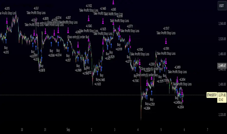
Innocent Heikin Ashi Ethereum StrategyHello there, im back!
If you are familiar with my previous scripts, this one will seem like the future's nostalgia!
Functionality:
As you can see, all candles are randomly colored. This has no deeper meaning, it should remind you to switch to Heikin Ashi. The Strategy works on standard candle stick charts, but should be used with Heikin Ashi to see the actual results. (Regular OHLC calculations are included.)
Same as in my previous scripts we import our PVSRA Data from @TradersReality open source Indicator.
With this data and the help of moving averages, we have got an edge in the market.
Signal Logic:
When a "violently green" candle appears (high buy volume + tick speed) above the 50 EMA indicates a change in trend and sudden higher prices. Depending on OHLC of the candle itself and volume, Take Profit and Stop Loss is calculated. (The price margin is the only adjustable setting). Additionally, to make this script as simple and easily useable as possible, all other adjustable variables have been already set to the best suitable value and the chart was kept plain, except for the actual entries and exits.
Basic Settings and Adjustables:
Main Input 1: TP and SL combined price range. (Double, Triple R:R equally.)
Trade Inputs: All standard trade size and contract settings for testing available.
Special Settings:
Checkbox 1: Calculate Signal in Heikin Ashi chart, including regular candle OHLC („Open, High, Low, Close“)
Checkbox 2/3: Calculate by order fill or every tick.
Checkbox 4: Possible to fill orders on bar close.
Timeframe and practical usage:
Made for the 5 Minute to 1 hour timeframe.
Literally ONLY works on Ethereum and more or less on Bitcoin.
EVERY other asset has absolute 0% profitability.
Have fun and share with your friends!
Thanks for using!
Example Chart:
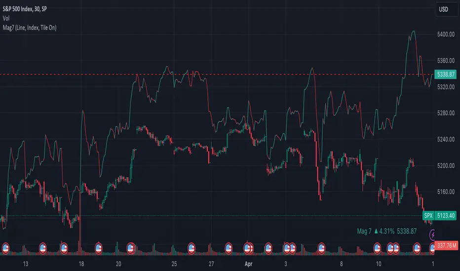
Mag7 IndexThis is an indicator index based on cumulative market value of the Magnificent 7 (AAPL, MSFT, NVDA, TSLA, META, AMZN, GOOG). Such an indicator for the famous Mag 7, against which your main security can be benchmarked, was missing from the TradingView user library.
The index bar values are calculated by taking the weighted average of the 7 stocks, relative to their market cap. Explicitly, we are multiplying each bar period's total outstanding stock amount by the OHLC of that period for each stock and dividing that value by the combined sum of outstanding stock for the 7 corporations. OHLC is taken for the extended trading session.
The index dynamically adjusts with respect to the chosen main security and the bars/line visible in the chart window; that is, the first close value is normalized to the main security's first close value. It provides recalculation of the performance in that chart window as you scroll (this isn't apparent in the demo chart above this description).
It can be useful for checking market breadth, or benchmarking price performance of the individual stock components that comprise the Magnificent 7. I prefer comparing the indicator to the Nasdaq Composite Index (IXIC) or S&P500 (SPX), but of course you can make comparisons to any security or commodity.
Settings Input Options:
1) Bar vs. Line - view as OHLC colored bars or line chart. Line chart color based on close above or below the previous period close as green or red line respectively.
2) % vs Regular - the final value for the window period as % return for that window or index value
3) Turn on/off - bottom right tile displaying window-period performance
Inspired by the simpler NQ 7 Index script by @RaenonX but with normalization to main security at start of window and additional settings input options.
Please provide feedback for additional features, e.g., if a regular/extended session option is useful.
ZigzagMethodsLibrary "ZigzagMethods"
Object oriented implementation of Zigzag methods. Please refer to ZigzagTypes library for User defined types used in this library
tostring(this, sortKeys, sortOrder, includeKeys)
Converts ZigzagTypes/Pivot object to string representation
Parameters:
this : ZigzagTypes/Pivot
sortKeys : If set to true, string output is sorted by keys.
sortOrder : Applicable only if sortKeys is set to true. Positive number will sort them in ascending order whreas negative numer will sort them in descending order. Passing 0 will not sort the keys
includeKeys : Array of string containing selective keys. Optional parmaeter. If not provided, all the keys are considered
Returns: string representation of ZigzagTypes/Pivot
tostring(this, sortKeys, sortOrder, includeKeys)
Converts Array of Pivot objects to string representation
Parameters:
this : Pivot object array
sortKeys : If set to true, string output is sorted by keys.
sortOrder : Applicable only if sortKeys is set to true. Positive number will sort them in ascending order whreas negative numer will sort them in descending order. Passing 0 will not sort the keys
includeKeys : Array of string containing selective keys. Optional parmaeter. If not provided, all the keys are considered
Returns: string representation of Pivot object array
tostring(this)
Converts ZigzagFlags object to string representation
Parameters:
this : ZigzagFlags object
Returns: string representation of ZigzagFlags
tostring(this, sortKeys, sortOrder, includeKeys)
Converts ZigzagTypes/Zigzag object to string representation
Parameters:
this : ZigzagTypes/Zigzagobject
sortKeys : If set to true, string output is sorted by keys.
sortOrder : Applicable only if sortKeys is set to true. Positive number will sort them in ascending order whreas negative numer will sort them in descending order. Passing 0 will not sort the keys
includeKeys : Array of string containing selective keys. Optional parmaeter. If not provided, all the keys are considered
Returns: string representation of ZigzagTypes/Zigzag
calculate(this, ohlc, indicators, indicatorNames)
Calculate zigzag based on input values and indicator values
Parameters:
this : Zigzag object
ohlc : Array containing OHLC values. Can also have custom values for which zigzag to be calculated
indicators : Array of indicator values
indicatorNames : Array of indicator names for which values are present. Size of indicators array should be equal to that of indicatorNames
Returns: current Zigzag object
calculate(this)
Calculate zigzag based on properties embedded within Zigzag object
Parameters:
this : Zigzag object
Returns: current Zigzag object
nextlevel(this)
Calculate Next Level Zigzag based on the current calculated zigzag object
Parameters:
this : Zigzag object
Returns: Next Level Zigzag object
clear(this)
Clears zigzag drawings array
Parameters:
this : array
Returns: void
drawfresh(this)
draws fresh zigzag based on properties embedded in ZigzagDrawing object
Parameters:
this : ZigzagDrawing object
Returns: ZigzagDrawing object
drawcontinuous(this)
draws zigzag based on the zigzagmatrix input
Parameters:
this : ZigzagDrawing object
Returns:

Magnifying Glass (LTF Candles) by SiddWolf█ OVERVIEW
This indicator displays The Lower TimeFrame Candles in current chart, Like Zooming in on the Candle to see it's Lower TimeFrame Structure. It plots intrabar OHLC data inside a Label along with the volume structure of LTF candle in an eloquent format.
█ QUICK GUIDE
Just apply it to the chart, Hover the mouse on the Label and ta-da you have a Lower Timeframe OHLC candles on your screen. Move the indicator to the top and shrink it all the way up, because all the useful data is inside the label.
Inside the label: The OHLC ltf candles are pretty straightforward. Volume strength of ltf candles is shown at bottom and Volume Profile on the left. Read the Details below for more information.
In the settings, you will find the option to change the UI and can play around with Lower TimeFrame Settings.
█ DETAILS
First of all, I would like to thank the @TradingView team for providing the function to get access to the lower timeframe data. It is because of them that this magical indicator came into existence.
Magnifying Glass indicator displays a Candle's Lower TimeFrame data in Higher timeframe chart. It displays the LTF candles inside a label. It also shows the Volume structure of the lower timeframe candles. Range percentage shown at the bottom is the percentage change between high and low of the current timeframe candle. LTF candle's timeframe is also shown at the bottom on the label.
This indicator is gonna be most useful to the price action traders, which is like every profitable trader.
How this indicator works:
I didn't find any better way to display ltf candles other than labels. Labels are not build for such a complex behaviour, it's a workaround to display this important information.
It gets the lower timeframe information of the candle and uses emojis to display information. The area that is shown, is the range of the current timeframe candle. Range is a difference between high and low of the candle. Range percentage is also shown at the bottom in the label.
I've divided the range area into 20 parts because there are limitation to display data in the labels. Then the code checks out, in what area does the ltf candle body or wick lies, then displays the information using emojis.
The code uses matrix elements for each block and relies heavily on string manipulation. But what I've found most difficult, is managing to fit everything correctly and beautifully so that the view doesn't break.
Volume Structure:
Strength of the Lower TimeFrame Candles is shown at the bottom inside the label. The Higher Volume is shown with the dark shade color and Lower Volume is shown with the light shade. The volume of candles are also ranked, with 1 being the highest volume, so you can see which candle have the maximum to minimum volume. This is pretty important to make a price action analysis of the lower timeframe candles.
Inside the label on the left side you will see the volume profile. As the volume on the bottom shows the strength of each ltf candles, Volume profile on the left shows strength in a particular zone. The Darker the color, the higher the volume in the zone. The Highest volume on the left represents Point of Control (Volume Profile POC) of the candle.
Lower TimeFrame Settings:
There is a limitation for the lowest timeframe you can show for a chart, because there is only so much data you can fit inside a label. A label can show upto 20 blocks of emojis (candle blocks) per row. Magnifying Glass utilizes this behaviour of labels. 16 blocks are used to display ltf candles, 1 for volume profile and two for Open and Close Highlighter.
So for any chart timeframe, ltf candles can be 16th part of htf candle. So 4 hours chart can show as low as 15 minutes of ltf data. I didn't provide the open settings for changing the lower timeframe, as it would give errors in a lot of ways. You can change the timeframe for each chart time from the settings provided.
Limitations:
Like I mentioned earlier, this indicator is a workaround to display ltf candles inside a label. This indicator does not work well on smaller screens. So if you are not able to see the label, zoom out on your browser a bit. Move the indicator to either top or bottom of all indicators and shrink it's space because all details are inside the label.
█ How I use MAGNIFYING GLASS:
This indicator provides you an edge, on top of your existing trading strategy. How you use Magnifying Glass is entirely dependent on your strategy.
I use this indicator to get a broad picture, before getting into a trade. For example I see a Doji or Engulfing or any other famous candlestick pattern on important levels, I hover the mouse on Magnifying Glass, to look for the price action the ltf candles have been through, to make that pattern. I also use it with my "Wick Pressure" indicator, to check price action at wick zones. Whenever I see price touching important supply and demand zones, I check last few candles to read chart like a beautiful price action story.
Also volume is pretty important too. This is what makes Magnifying Glass even better than actual lower timeframe candles. The increasing volume along with up/down trend price shows upward/downward momentum. The sudden burst (peak) in the volume suggests volume climax.
Volume profile on the left can be interpreted as the strength/weakness zones inside a candle. The low volume in a price zone suggests weakness and High volume suggests strength. The Highest volume on the left act as POC for that candle.
Before making any trade, I read the structure of last three or four candles to get the complete price action picture.
█ Conclusion
Magnifying Glass is a well crafted indicator that can be used to track lower timeframe price action. This indicator gives you an edge with the Multi Timeframe Analysis, which I believe is the most important aspect of profitable trading.
~ @SiddWolf

Rolling Heikin Ashi Candles█ OVERVIEW
This indicator displays a Rolling Heikin Ashi Candles for a given timeframe Multiplier. Contrary to Heikin Ashi Candles Charts, if the timeframe Multiplier is "5", this indicator plots Heikin Ashi Candles OHLC of the last 5 Candles.
█ WHAT IS THE NEED FOR IT
Let's see if we want to use a Higher timeframe OHLC Data using security function or resolution options. The indicator repaints until the higher timeframe Heikin Ashi Candles closes, leading to a repainting strategy or indicator using higher-timeframe data. So we can use Rolling Heikin Ashi Candles in these cases.
█ USES
To Pull out higher timeframe Heikin Ashi Candles OHLC Data to build a non-repainting strategy or indicator.
█ WHY I AM BUILDING THIS SIMPLE INDICATOR
There is no doubt higher timeframe analysis is a critical study to mastering the markets.
I found a necessity for an indicator that analyses multiple higher timeframes and gives us a cumulative or average trend direction. I already built the indicator; I will release it soon. The Indicator I am building is wholly based on my understanding and perspective of Market Structure. Please use this indicator idea to remove the repainting issue when you make an indicator that utilises higher timeframe data.
I am using this in my upcoming indicators. Felt to share before head.
Stay Tuned...
If you have any recommendations or alternative ideas, then please drop a comment under the script ;)

MrBS:Directional Movement Index [Trend Friend Strategy]This goes with my MrBS:DMI+ indicator. I originally combined them into one, but then you cannot set alerts based on what the ADX and DMI is doing, only strategy alerts, so separate ones have more flexibility and uses.
Indicator Version is found under "MrBS:Directional Movement Index " ()
//// THE IDEA
The majority of profits made in the market come from trending markets. Of course there are strategies that would say otherwise but for the majority of people, THE TREND IS YOUR FRIEND (until the end). The idea is to follow the trend, entering once it has established its self and exiting positions when the trend weakens. This strategy gives a rough idea of the returns produced from following purely the ADX signals. At first Heikin Ashi values were used for the calculation but the results show it's not that effective. The functionality to switch between calculation types has been left in, so we can uses HA candle data to generate signals from while looking at an OHLC chart, if we want to experiment. Due to the way strategies work, we are unable to get reliable results when running the strategy on the HA chart even if we are calculating the signals from the real OHLC values. It is best to always run strategies on standard charts.
When using this strategy, I look for confirmation of the signal based on stochastic (14:3:6) direction, reversal level of stochastic, and divergance, to add confidence and adjust position size accordingly. I am going to try and code some version of that in future updates, if anyone can help or has suggestions please drop me a message.
//// INDICATOR DETAILS
- The default settings are for optimized Daily charts, for 4 hour I would suggest a smoothing of 2.
- The default values used for calculation are the Real OHLC, we can change this to Heikin Ashi in the menu.
- The strategy enters a position when ADX crosses the threshold level, and closes the position when ADX starts to fall.
- There is a signal filter in the form of a 377 period Hull Moving Average, which the price must be above or bellow for long and short positions respectively.
- The strategy closes the position when a cross-under of the ADX and its 4 period EMA. This is an attempt to stay into positions longer as sometimes the ADX will fall for 1 bar and then keep rising, while the overall trend is strong. The downside to this is that we exit trades later and this affects our max drawdown.

Difference over barsDescription:
One of my followers asked about an indicator that shows the difference between the open and a previous close and didn't find one so I wrote this one. This is similar to a momentum indicator except it offers more flexibility. While the standard momentum indicator calculates a difference between current close and a previous close (sometimes customizable to work on open, high or lows instead of close), this allows to mix and match between open, high, low and close. It also offers multiple kinds of moving averages.
Settings:
Current point of reference
Previous point of reference
Difference over how many bars?
How it works:
The indicator calculates the difference between the current point of reference and a previous (n-bars back) point of reference (where n is given by the "Difference over how many bars?").
How to use it:
find historical support lines like the 0.68 line in the cart above where in the past the indicator tends to bounce back; similarly find resistance lines like the -0.75 line in the chart (which servers as a resistance line both for the main indicator line and its moving average )
look for convergence between the price and the indicator; for example, if the price is going up and the indicator is going down a change in the price direction may be coming soon
look for the indicator crossing its moving average: moving up will signify an up trend and vice-versa
since the difference between the open and previous close (which is what the blue line in the chart shows) since to go up to 0.68 (the upper horizontal line) and down to -0.75 (the lower horizontal line) most of the time, one strategy, using options, is to to buy, right before the close of a trading day, a "long iron butterfly": buy-to-open (BTO) both a call and a put at the strike price and sell-to-open (STO) a call at a strike of around $0.68 more and sell to open a put at a strike of around $0.75 less. The STO legs should be for the next expiration and the BTO legs for the next expiration after that. This way the STO will decrease their time value faster than the BTO legs if the price stays flat (which plays to your advantage) and the BTO legs may make profit if the next day it opens away from the price at which the ticker closed the previous day (when the position was opened). The most profit is when it moves right up to one of the STO legs. This position would normally be closed next day at opening. The percentage of profit it makes is low compared to other strategies but also the percentage of the total cost at risk is also low which could potentially allow a trader to increase the lot and thus, in the end, the total profit amount may be comparable to other strategies.
Notes:
The indicator in the chart above comes with the standard options. For a more standard momentum indicator set both the current and previous reference point to the same OHLC value (such as "close").
The 0.68 and -0.75 levels are for open/close (current/previous point of reference) for ticker INTC. Obviously, other tickers will likely have other levels and you will have to find those yourself. If you use INTC but use other combination of current and previous reference points, they will have different levels as well.

Market EKGShort Summary
This indicator takes the differences in the previous 4 period OHLC inputs, and compares them to the previously closed candle input. The difference is then placed into an oscillator that when all four inputs are scrolled back on, shows an EKG appearing oscillator / volatility measure for traders to use on indexes, tickers and markets that do not allow typical volume based indicators.
Full Summary
Named for its similar appearance to an EKG medical chart, this script takes the difference in relative averages of previous periods in a trend , and compares it to the most recent period input. This can be used as a price based volatility measure, useful in markets that may be limited by no valume measures or other indexes where volatility is useful to meeasure but will not allow volume initializations.
Steps taken
Taking Previous Period OHLC
Taking Previous 3 Periods OHLC Avgs
Difference Between #1 & #2 (Comparing most recent confirmation to relative trend
Plot Results
This RSI Script is intended for public use and can be shared / implemented as needed
Questions? I do not monitor my TradingView inbox. See email address in signature at the bottom of this page for contact information.
Use this script and its calculations as needed! No permission required.
Cheers,
[PX] M/W/D LevelHey guys,
this script shows monthly, weekly and daily OHLC data represented as horizontal level.
I tried to make it as user-friendly as possible. Therefore, you can add different colors and styles for each level, as well as turn them on and off.
With the "Label Offset" -parameter you are in control where the label text should appear. You can shift it from left to right and vice-versa. To shift it to the left choose a negative value. To shift it to the right use a positive one.
This best setting for me personally is the "Candle Selection" -dropdown. This allows you to decide wether you want to show the previous candles OHLC-data or the current live OHLC-data.
!!CAUTION!! If you use the "Current Month/Week/Day" -selection be aware that values shown are "live"-data of the current candle. Therefore, values will change the same way your chart keeps changing on live data.
The "Previous Month/Week/Day" -selection on the other hand is historical data and therefore only changes once we reached a new month/week/day.
If you like my work, consider leaving a like :)
Happy trading!
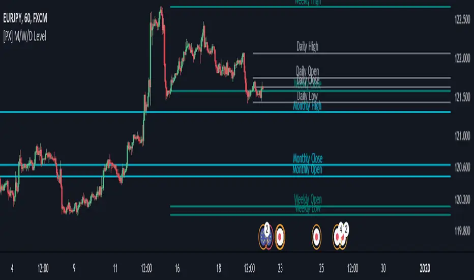
Chiki-Poki BFXLS Longs Shorts Abs Normalized Volume Pro by RRBChiki-Poki BFXLS Longs vs Shorts Absolute Normalized Volume Value Pro by RagingRocketBull 2018
Version 1.0
This indicator displays Longs vs Shorts in a side by side graph, shows volume's absolute price value and normalized volume of Longs/Shorts for the current asset. This allows for more accurate L/S comparisons (like a log scale for volume) since volume on spot exchanges (Bitstamp, Bitfinex, Coinbase etc) is measured in coins traded, not USD traded. Similarly, L/S is usually the amount of coins in open L/S positions, not their total USD value. On Bitmex and other futures exchanges volume is measured in USD traded, so you don't need to apply the Volume Absolute Price Value checkbox to compare L/S. You should always check first whether your source is measured in coins or USD.
Chiki-Poki BFXLS primarily uses *SHORTS/LONGS feeds from Bitfinex for the current crypto asset, but you can specify custom L/S source tickers instead.
This 2-in-1 works both in the Main Chart and in the indicator pane below. You can switch between Main/Sub Window panes using RMB on the indicator's name and selecting Move To/Pane Above/Below.
This indicator doesn't use volume of the current asset. It uses L/S ticker's OHLC as a source for SHORTS/LONGS volumes instead. Essentially L/S => L/S Volume == L/S
Features:
- Display Longs vs Shorts side by side graph for the current crypto asset, i.e. for BTCUSD - BTCUSDLONGS/BTCUSDSHORTS, for ETHUSD - ETHUSDLONGS/ETHUSDSHORTS etc.
- Use custom OHLC ticker sources for Longs/Shorts from different exchanges/crypto assets with/without exchange prefix.
- Plot Longs/Shorts as lines or candles
- Show/Hide L/S, Diff, MAs, ATH/ATL
- Use Longs/Shorts Volume Absolute Price Value (Price * L/S Volume) instead of Coins Traded in open L/S positions to compare total L/S value/capitalization
- Normalize L/S Volume using Price / Price MA / L/S Volume MA
- Supports any existing type of MA: SMA, EMA, WMA, HMA etc
- Volume Absolute Price Value / Normalize also works on candles
- Oscillator mode with negative axis (works in both Main Chart/Subwindow panes).
- Highlight L/S Volume spikes above L/S MAs in both lines/oscillator.
- Change L/S MA color based on a number of last rising/falling L/S bars, colorize candles
- Display L/S volume as 1000s, mlns, or blns using alpha multiplier
1. based on BFXLS Longs vs Shorts and Compare Style, uses plot*, security and custom hma functions
2. swma has a fixed length = 4, alma and linreg have additional offset and smoothing params
Notes:
- Make sure that Left Price Scale shows up with Auto Fit Data enabled. You can reattach indicator to a different scale in Style.
- It is not recommended to switch modes multiple times due to TradingView's scale reattachment bugs. You should switch between Main Chart and Sub Window only once.
- When the USD price of an asset is lower you can trade more coins but capitalization value won't be as significant as when there are less coins for a higher price. Same goes for Shorts/Longs.
Current ATH in shorts doesn't trigger a squeeze because its total value is now far less than before and we are in a bear market where it's normal to have a higher number of shorts.
- You should always subtract Hedged L/S from L/S because hedged positions are temporary - used to preserve the value of the main position in the opposite direction and should be disregarded as such.
- Low margin rates increase the probability of a move in an underlying direction because it is cheaper. High margin rates => the market is anticipating a move in this direction, thus a more expensive rate. Sudden 5-10x rate raises imply a possible reversal soon. high - 0.1%, avg - 0.01-0.02%, low - 0.001-0.005%
You can also check out:
- BFXLS Longs/Shorts on BFXData
- Bitfinex L/S margin rates and Hedged L/S on datamish
- Bitmex L/S on Coinfarm.online