Reversal Point Dynamics - Machine Learning⇋ Reversal Point Dynamics - Machine Learning
RPD Machine Learning: Self-Adaptive Multi-Armed Bandit Trading System
RPD Machine Learning is an advanced algorithmic trading system that implements genuine machine learning through contextual multi-armed bandits, reinforcement learning, and online adaptation. Unlike traditional indicators that use fixed rules, RPD learns from every trade outcome , automatically discovers which strategies work in current market conditions, and continuously adapts without manual intervention .
Core Innovation: The system deploys six distinct trading policies (ranging from aggressive trend-following to conservative range-bound strategies) and uses LinUCB contextual bandit algorithms with Random Fourier Features to learn which policy performs best in each market regime. After the initial learning phase (50-100 trades), the system achieves autonomous adaptation , automatically shifting between policies as market conditions evolve.
Target Users: Quantitative traders, algorithmic trading developers, systematic traders, and data-driven investors who want a system that adapts over time . Suitable for stocks, futures, forex, and cryptocurrency on any liquid instrument with >100k daily volume.
The Problem This System Solves
Traditional Technical Analysis Limitations
Most trading systems suffer from three fundamental challenges :
Fixed Parameters: Static settings (like "buy when RSI < 30") work well in backtests but may struggle when markets change character. What worked in low-volatility environments may not work in high-volatility regimes.
Strategy Degradation: Manual optimization (curve-fitting) produces systems that perform well on historical data but may underperform in live trading. The system never adapts to new market conditions.
Cognitive Overload: Running multiple strategies simultaneously forces traders to manually decide which one to trust. This leads to hesitation, late entries, and inconsistent execution.
How RPD Machine Learning Addresses These Challenges
Automated Strategy Selection: Instead of requiring you to choose between trend-following and mean-reversion strategies, RPD runs all six policies simultaneously and uses machine learning to automatically select the best one for current conditions. The decision happens algorithmically, removing human hesitation.
Continuous Learning: After every trade, the system updates its understanding of which policies are working. If the market shifts from trending to ranging, RPD automatically detects this through changing performance patterns and adjusts selection accordingly.
Context-Aware Decisions: Unlike simple voting systems that treat all conditions equally, RPD analyzes market context (ADX regime, entropy levels, volatility state, volume patterns, time of day, historical performance) and learns which combinations of context features correlate with policy success.
Machine Learning Architecture: What Makes This "Real" ML
Component 1: Contextual Multi-Armed Bandits (LinUCB)
What Is a Multi-Armed Bandit Problem?
Imagine facing six slot machines, each with unknown payout rates. The exploration-exploitation dilemma asks: Should you keep pulling the machine that's worked well (exploitation) or try others that might be better (exploration)? RPD solves this for trading policies.
Academic Foundation:
RPD implements Linear Upper Confidence Bound (LinUCB) from the research paper "A Contextual-Bandit Approach to Personalized News Article Recommendation" (Li et al., 2010, WWW Conference). This algorithm is used in content recommendation and ad placement systems.
How It Works:
Each policy (AggressiveTrend, ConservativeRange, VolatilityBreakout, etc.) is treated as an "arm." The system maintains:
Reward History: Tracks wins/losses for each policy
Contextual Features: Current market state (8-10 features including ADX, entropy, volatility, volume)
Uncertainty Estimates: Confidence in each policy's performance
UCB Formula: predicted_reward + α × uncertainty
The system selects the policy with highest UCB score , balancing proven performance (predicted_reward) with potential for discovery (uncertainty bonus). Initially, all policies have high uncertainty, so the system explores broadly. After 50-100 trades, uncertainty decreases, and the system focuses on known-performing policies.
Why This Matters:
Traditional systems pick strategies based on historical backtests or user preference. RPD learns from actual outcomes in your specific market, on your timeframe, with your execution characteristics.
Component 2: Random Fourier Features (RFF)
The Non-Linearity Challenge:
Market relationships are often non-linear. High ADX may indicate favorable conditions when volatility is normal, but unfavorable when volatility spikes. Simple linear models struggle to capture these interactions.
Academic Foundation:
RPD implements Random Fourier Features from "Random Features for Large-Scale Kernel Machines" (Rahimi & Recht, 2007, NIPS). This technique approximates kernel methods (like Support Vector Machines) while maintaining computational efficiency for real-time trading.
How It Works:
The system transforms base features (ADX, entropy, volatility, etc.) into a higher-dimensional space using random projections and cosine transformations:
Input: 8 base features
Projection: Through random Gaussian weights
Transformation: cos(W×features + b)
Output: 16 RFF dimensions
This allows the bandit to learn non-linear relationships between market context and policy success. For example: "AggressiveTrend performs well when ADX >25 AND entropy <0.6 AND hour >9" becomes naturally encoded in the RFF space.
Why This Matters:
Without RFF, the system could only learn "this policy has X% historical performance." With RFF, it learns "this policy performs differently in these specific contexts" - enabling more nuanced selection.
Component 3: Reinforcement Learning Stack
Beyond bandits, RPD implements a complete RL framework :
Q-Learning: Value-based RL that learns state-action values. Maps 54 discrete market states (trend×volatility×RSI×volume combinations) to 5 actions (4 policies + no-trade). Updates via Bellman equation after each trade. Converges toward optimal policy after 100-200 trades.
TD(λ) with Eligibility Traces: Extension of Q-Learning that propagates credit backwards through time . When a trade produces an outcome, TD(λ) updates not just the final state-action but all states visited during the trade, weighted by eligibility decay (λ=0.90). This accelerates learning from multi-bar trades.
Policy Gradient (REINFORCE): Learns a stochastic policy directly from 12 continuous market features without discretization. Uses gradient ascent to increase probability of actions that led to positive outcomes. Includes baseline (average reward) for variance reduction.
Meta-Learning: The system learns how to learn by adapting its own learning rates based on feature stability and correlation with outcomes. If a feature (like volume ratio) consistently correlates with success, its learning rate increases. If unstable, rate decreases.
Why This Matters:
Q-Learning provides fast discrete decisions. Policy Gradient handles continuous features. TD(λ) accelerates learning. Meta-learning optimizes the optimization. Together, they create a robust, multi-approach learning system that adapts more quickly than any single algorithm.
Component 4: Policy Momentum Tracking (v2 Feature)
The Recency Challenge:
Standard bandits treat all historical data equally. If a policy performed well historically but struggles in current conditions due to regime shift, the system may be slow to adapt because historical success outweighs recent underperformance.
RPD's Solution:
Each policy maintains a ring buffer of the last 10 outcomes. The system calculates:
Momentum: recent_win_rate - global_win_rate (range: -1 to +1)
Confidence: consistency of recent results (1 - variance)
Policies with positive momentum (recent outperformance) get an exploration bonus. Policies with negative momentum and high confidence (consistent recent underperformance) receive a selection penalty.
Effect: When markets shift, the system detects the shift more quickly through momentum tracking, enabling faster adaptation than standard bandits.
Signal Generation: The Core Algorithm
Multi-Timeframe Fractal Detection
RPD identifies reversal points using three complementary methods :
1. Quantum State Analysis:
Divides price range into discrete states (default: 6 levels)
Peak signals require price in top states (≥ state 5)
Valley signals require price in bottom states (≤ state 1)
Prevents mid-range signals that may struggle in strong trends
2. Fractal Geometry:
Identifies swing highs/lows using configurable fractal strength
Confirms local extremum with neighboring bars
Validates reversal only if price crosses prior extreme
3. Multi-Timeframe Confirmation:
Analyzes higher timeframe (4× default) for alignment
MTF confirmation adds probability bonus
Designed to reduce false signals while preserving valid setups
Probability Scoring System
Each signal receives a dynamic probability score (40-99%) based on:
Base Components:
Trend Strength: EMA(velocity) / ATR × 30 points
Entropy Quality: (1 - entropy) × 10 points
Starting baseline: 40 points
Enhancement Bonuses:
Divergence Detection: +20 points (price/momentum divergence)
RSI Extremes: +8 points (RSI >65 for peaks, <40 for valleys)
Volume Confirmation: +5 points (volume >1.2× average)
Adaptive Momentum: +10 points (strong directional velocity)
MTF Alignment: +12 points (higher timeframe confirms)
Range Factor: (high-low)/ATR × 3 - 1.5 points (volatility adjustment)
Regime Bonus: +8 points (trending ADX >25 with directional agreement)
Penalties:
High Entropy: -5 points (entropy >0.85, chaotic price action)
Consolidation Regime: -10 points (ADX <20, no directional conviction)
Final Score: Clamped to 40-99% range, classified as ELITE (>85%), STRONG (75-85%), GOOD (65-75%), or FAIR (<65%)
Entropy-Based Quality Filter
What Is Entropy?
Entropy measures randomness in price changes . Low entropy indicates orderly, directional moves. High entropy indicates chaotic, unpredictable conditions.
Calculation:
Count up/down price changes over adaptive period
Calculate probability: p = ups / total_changes
Shannon entropy: -p×log(p) - (1-p)×log(1-p)
Normalized to 0-1 range
Application:
Entropy <0.5: Highly ordered (ELITE signals possible)
Entropy 0.5-0.75: Mixed (GOOD signals)
Entropy >0.85: Chaotic (signals blocked or heavily penalized)
Why This Matters:
Prevents trading during choppy, news-driven conditions where technical patterns may be less reliable. Automatically raises quality bar when market is unpredictable.
Regime Detection & Market Microstructure - ADX-Based Regime Classification
RPD uses Wilder's Average Directional Index to classify markets:
Bull Trend: ADX >25, +DI > -DI (directional conviction bullish)
Bear Trend: ADX >25, +DI < -DI (directional conviction bearish)
Consolidation: ADX <20 (no directional conviction)
Transitional: ADX 20-25 (forming direction, ambiguous)
Filter Logic:
Blocks all signals during Transitional regime (avoids trading during uncertain conditions)
Blocks Consolidation signals unless ADX ≥ Min Trend Strength
Adds probability bonus during strong trends (ADX >30)
Effect: Designed to reduce signal frequency while focusing on higher-quality setups.
Divergence Detection
Bearish Divergence:
Price makes higher high
Velocity (price momentum) makes lower high
Indicates weakening upward pressure → SHORT signal quality boost
Bullish Divergence:
Price makes lower low
Velocity makes higher low
Indicates weakening downward pressure → LONG signal quality boost
Bonus: Adds probability points and additional acceleration factor. Divergence signals have historically shown higher success rates in testing.
Hierarchical Policy System - The Six Trading Policies
1. AggressiveTrend (Policy 0):
Probability Threshold: 60% (trades more frequently)
Entropy Threshold: 0.70 (tolerates moderate chaos)
Stop Multiplier: 2.5× ATR (wider stops for trends)
Target Multiplier: 5.0R (larger targets)
Entry Mode: Pyramid (scales into winners)
Best For: Strong trending markets, breakouts, momentum continuation
2. ConservativeRange (Policy 1):
Probability Threshold: 75% (more selective)
Entropy Threshold: 0.60 (requires order)
Stop Multiplier: 1.8× ATR (tighter stops)
Target Multiplier: 3.0R (modest targets)
Entry Mode: Single (one-shot entries)
Best For: Range-bound markets, low volatility, mean reversion
3. VolatilityBreakout (Policy 2):
Probability Threshold: 65% (moderate)
Entropy Threshold: 0.80 (accepts high entropy)
Stop Multiplier: 3.0× ATR (wider stops)
Target Multiplier: 6.0R (larger targets)
Entry Mode: Tiered (splits entry)
Best For: Compression breakouts, post-consolidation moves, gap opens
4. EntropyScalp (Policy 3):
Probability Threshold: 80% (very selective)
Entropy Threshold: 0.40 (requires extreme order)
Stop Multiplier: 1.5× ATR (tightest stops)
Target Multiplier: 2.5R (quick targets)
Entry Mode: Single
Best For: Low-volatility grinding moves, tight ranges, highly predictable patterns
5. DivergenceHunter (Policy 4):
Probability Threshold: 70% (quality-focused)
Entropy Threshold: 0.65 (balanced)
Stop Multiplier: 2.2× ATR (moderate stops)
Target Multiplier: 4.5R (balanced targets)
Entry Mode: Tiered
Best For: Divergence-confirmed reversals, exhaustion moves, trend climax
6. AdaptiveBlend (Policy 5):
Probability Threshold: 68% (balanced)
Entropy Threshold: 0.75 (balanced)
Stop Multiplier: 2.0× ATR (standard)
Target Multiplier: 4.0R (standard)
Entry Mode: Single
Best For: Mixed conditions, general trading, fallback when no clear regime
Policy Clustering (Advanced/Extreme Modes)
Policies are grouped into three clusters based on regime affinity:
Cluster 1 (Trending): AggressiveTrend, DivergenceHunter
High regime affinity (0.8): Performs well when ADX >25
Moderate vol affinity (0.6): Works in various volatility
Cluster 2 (Ranging): ConservativeRange, AdaptiveBlend
Low regime affinity (0.3): Better suited for ADX <20
Low vol affinity (0.4): Optimized for calm markets
Cluster 3 (Breakout): VolatilityBreakout
Moderate regime affinity (0.6): Works in multiple regimes
High vol affinity (0.9): Requires high volatility for optimal characteristics
Hierarchical Selection Process:
Calculate cluster scores based on current regime and volatility
Select best-matching cluster
Run UCB selection within chosen cluster
Apply momentum boost/penalty
This two-stage process reduces learning time - instead of choosing among 6 policies from scratch, system first narrows to 1-2 policies per cluster, then optimizes within cluster.
Risk Management & Position Sizing
Dynamic Kelly Criterion Sizing (Optional)
Traditional Fixed Sizing Challenge:
Using the same position size for all signal probabilities may be suboptimal. Higher-probability signals could justify larger positions, lower-probability signals smaller positions.
Kelly Formula:
f = (p × b - q) / b
Where:
p = win probability (from signal score)
q = loss probability (1 - p)
b = win/loss ratio (average_win / average_loss)
f = fraction of capital to risk
RPD Implementation:
Uses Fractional Kelly (1/4 Kelly default) for safety. Full Kelly is theoretically optimal but can recommend large position sizes. Fractional Kelly reduces volatility while maintaining adaptive sizing benefits.
Enhancements:
Probability Bonus: Normalize(prob, 65, 95) × 0.5 multiplier
Divergence Bonus: Additional sizing on divergence signals
Regime Bonus: Additional sizing during strong trends (ADX >30)
Momentum Adjustment: Hot policies receive sizing boost, cold policies receive reduction
Safety Rails:
Minimum: 1 contract (floor)
Maximum: User-defined cap (default 10 contracts)
Portfolio Heat: Max total risk across all positions (default 4% equity)
Multi-Mode Stop Loss System
ATR Mode (Default):
Stop = entry ± (ATR × base_mult × policy_mult)
Consistent risk sizing
Ignores market structure
Best for: Futures, forex, algorithmic trading
Structural Mode:
Finds swing low (long) or high (short) over last 20 bars
Identifies fractal pivots within lookback
Places stop below/above structure + buffer (0.1× ATR)
Best for: Stocks, instruments that respect structure
Hybrid Mode (Intelligent):
Attempts structural stop first
Falls back to ATR if:
Structural level is invalid (beyond entry)
Structural stop >2× ATR away (too wide)
Best for: Mixed instruments, adaptability
Dynamic Adjustments:
Breakeven: Move stop to entry + 1 tick after 1.0R profit
Trailing: Trail stop 0.8R behind price after 1.5R profit
Timeout: Force close after 30 bars (optional)
Tiered Entry System
Challenge: Equal sizing on all signals may not optimize capital allocation relative to signal quality.
Solution:
Tier 1 (40% of size): Enters immediately on all signals
Tier 2 (60% of size): Enters only if probability ≥ Tier 2 trigger (default 75%)
Example:
Calculated optimal size: 10 contracts
Signal probability: 72%
Tier 2 trigger: 75%
Result: Enter 4 contracts only (Tier 1)
Same signal at 80% probability
Result: Enter 10 contracts (4 Tier 1 + 6 Tier 2)
Effect: Automatically scales size to signal quality, optimizing capital allocation.
Performance Optimization & Learning Curve
Warmup Phase (First 50 Trades)
Purpose: Ensure all policies get tested before system focuses on preferred strategies.
Modifications During Warmup:
Probability thresholds reduced 20% (65% becomes 52%)
Entropy thresholds increased 20% (more permissive)
Exploration rate stays high (30%)
Confidence width (α) doubled (more exploration)
Why This Matters:
Without warmup, system might commit to early-performing policy without testing alternatives. Warmup forces thorough exploration before focusing on best-performing strategies.
Curriculum Learning
Phase 1 (Trades 1-50): Exploration
Warmup active
All policies tested
High exploration (30%)
Learning fundamental patterns
Phase 2 (Trades 50-100): Refinement
Warmup ended, thresholds normalize
Exploration decaying (30% → 15%)
Policy preferences emerging
Meta-learning optimizing
Phase 3 (Trades 100-200): Specialization
Exploration low (15% → 8%)
Clear policy preferences established
Momentum tracking fully active
System focusing on learned patterns
Phase 4 (Trades 200+): Maturity
Exploration minimal (8% → 5%)
Regime-policy relationships learned
Auto-adaptation to market shifts
Stable performance expected
Convergence Indicators
System is learning well when:
Policy switch rate decreasing over time (initially ~50%, should drop to <20%)
Exploration rate decaying smoothly (30% → 5%)
One or two policies emerge with >50% selection frequency
Performance metrics stabilizing over time
Consistent behavior in similar market conditions
System may need adjustment when:
Policy switch rate >40% after 100 trades (excessive exploration)
Exploration rate not decaying (parameter issue)
All policies showing similar selection (not differentiating)
Performance declining despite relaxed thresholds (underlying signal issue)
Highly erratic behavior after learning phase
Advanced Features
Attention Mechanism (Extreme Mode)
Challenge: Not all features are equally important. Trading hour might matter more than price-volume correlation, but standard approaches treat them equally.
Solution:
Each RFF dimension has an importance weight . After each trade:
Calculate correlation: sign(feature - 0.5) × sign(reward)
Update importance: importance += correlation × 0.01
Clamp to range
Effect: Important features get amplified in RFF transformation, less important features get suppressed. System learns which features correlate with successful outcomes.
Temporal Context (Extreme Mode)
Challenge: Current market state alone may be incomplete. Historical context (was volatility rising or falling?) provides additional information.
Solution:
Includes 3-period historical context with exponential decay (0.85):
Current features (weight 1.0)
1 bar ago (weight 0.85)
2 bars ago (weight 0.72)
Effect: Captures momentum and acceleration of market features. System learns patterns like "rising volatility with falling entropy" that may precede significant moves.
Transfer Learning via Episodic Memory
Short-Term Memory (STM):
Last 20 trades
Fast adaptation to immediate regime
High learning rate
Long-Term Memory (LTM):
Condensed historical patterns
Preserved knowledge from past regimes
Low learning rate
Transfer Mechanism:
When STM fills (20 trades), patterns consolidated into LTM . When similar regime recurs later, LTM provides faster adaptation than starting from scratch.
Practical Implementation Guide - Recommended Settings by Instrument
Futures (ES, NQ, CL):
Adaptive Period: 20-25
ML Mode: Advanced
RFF Dimensions: 16
Policies: 6
Base Risk: 1.5%
Stop Mode: ATR or Hybrid
Timeframe: 5-15 min
Forex Majors (EURUSD, GBPUSD):
Adaptive Period: 25-30
ML Mode: Advanced
RFF Dimensions: 16
Policies: 6
Base Risk: 1.0-1.5%
Stop Mode: ATR
Timeframe: 5-30 min
Cryptocurrency (BTC, ETH):
Adaptive Period: 20-25
ML Mode: Extreme (handles non-stationarity)
RFF Dimensions: 32 (captures complexity)
Policies: 6
Base Risk: 1.0% (volatility consideration)
Stop Mode: Hybrid
Timeframe: 15 min - 4 hr
Stocks (Large Cap):
Adaptive Period: 25-30
ML Mode: Advanced
RFF Dimensions: 16
Policies: 5-6
Base Risk: 1.5-2.0%
Stop Mode: Structural or Hybrid
Timeframe: 15 min - Daily
Scaling Strategy
Phase 1 (Testing - First 50 Trades):
Max Contracts: 1-2
Goal: Validate system on your instrument
Monitor: Performance stabilization, learning progress
Phase 2 (Validation - Trades 50-100):
Max Contracts: 2-3
Goal: Confirm learning convergence
Monitor: Policy stability, exploration decay
Phase 3 (Scaling - Trades 100-200):
Max Contracts: 3-5
Enable: Kelly sizing (1/4 Kelly)
Goal: Optimize capital efficiency
Monitor: Risk-adjusted returns
Phase 4 (Full Deployment - Trades 200+):
Max Contracts: 5-10
Enable: Full momentum tracking
Goal: Sustained consistent performance
Monitor: Ongoing adaptation quality
Limitations & Disclaimers
Statistical Limitations
Learning Sample Size: System requires minimum 50-100 trades for basic convergence, 200+ trades for robust learning. Early performance (first 50 trades) may not reflect mature system behavior.
Non-Stationarity Risk: Markets change over time. A system trained on one market regime may need time to adapt when conditions shift (typically 30-50 trades for adjustment).
Overfitting Possibility: With 16-32 RFF dimensions and 6 policies, system has substantial parameter space. Small sample sizes (<200 trades) increase overfitting risk. Mitigated by regularization (λ) and fractional Kelly sizing.
Technical Limitations
Computational Complexity: Extreme mode with 32 RFF dimensions, 6 policies, and full RL stack requires significant computation. May perform slowly on lower-end systems or with many other indicators loaded.
Pine Script Constraints:
No true matrix inversion (uses diagonal approximation for LinUCB)
No cryptographic RNG (uses market data as entropy)
No proper random number generation for RFF (uses deterministic pseudo-random)
These approximations reduce mathematical precision compared to academic implementations but remain functional for trading applications.
Data Requirements: Needs clean OHLCV data. Missing bars, gaps, or low liquidity (<100k daily volume) can degrade signal quality.
Forward-Looking Bias Disclaimer
Reward Calculation Uses Future Data: The RL system evaluates trades using an 8-bar forward-looking window. This means when a position enters at bar 100, the reward calculation considers price movement through bar 108.
Why This is Disclosed:
Entry signals do NOT look ahead - decisions use only data up to entry bar
Forward data used for learning only, not signal generation
In live trading, system learns identically as bars unfold in real-time
Simulates natural learning process (outcomes are only known after trades complete)
Implication: Backtested metrics reflect this 8-bar evaluation window. Live performance may vary if:
- Positions held longer than 8 bars
- Slippage/commissions differ from backtest settings
- Market microstructure changes (wider spreads, different execution quality)
Risk Warnings
No Guarantee of Profit: All trading involves substantial risk of loss. Machine learning systems can fail if market structure fundamentally changes or during unprecedented events.
Maximum Drawdown: With 1.5% base risk and 4% max total risk, expect potential drawdowns. Historical drawdowns do not predict future drawdowns. Extreme market conditions can exceed expectations.
Black Swan Events: System has not been tested under: flash crashes, trading halts, circuit breakers, major geopolitical shocks, or other extreme events. Such events can exceed stop losses and cause significant losses.
Leverage Risk: Futures and forex involve leverage. Adverse moves combined with leverage can result in losses exceeding initial investment. Use appropriate position sizing for your risk tolerance.
System Failures: Code bugs, broker API failures, internet outages, or exchange issues can prevent proper execution. Always monitor automated systems and maintain appropriate safeguards.
Appropriate Use
This System Is:
✅ A machine learning framework for adaptive strategy selection
✅ A signal generation system with probabilistic scoring
✅ A risk management system with dynamic sizing
✅ A learning system designed to adapt over time
This System Is NOT:
❌ A price prediction system (does not forecast exact prices)
❌ A guarantee of profits (can and will experience losses)
❌ A replacement for due diligence (requires monitoring and understanding)
❌ Suitable for complete beginners (requires understanding of ML concepts, risk management, and trading fundamentals)
Recommended Use:
Paper trade for 100 signals before risking capital
Start with minimal position sizing (1-2 contracts) regardless of calculated size
Monitor learning progress via dashboard
Scale gradually over several months only after consistent results
Combine with fundamental analysis and broader market context
Set account-level risk limits (e.g., maximum drawdown threshold)
Never risk more than you can afford to lose
What Makes This System Different
RPD implements academically-derived machine learning algorithms rather than simple mathematical calculations or optimization:
✅ LinUCB Contextual Bandits - Algorithm from WWW 2010 conference (Li et al.)
✅ Random Fourier Features - Kernel approximation from NIPS 2007 (Rahimi & Recht)
✅ Q-Learning, TD(λ), REINFORCE - Standard RL algorithms from Sutton & Barto textbook
✅ Meta-Learning - Learning rate adaptation based on feature correlation
✅ Online Learning - Real-time updates from streaming data
✅ Hierarchical Policies - Two-stage selection with clustering
✅ Momentum Tracking - Recent performance analysis for faster adaptation
✅ Attention Mechanism - Feature importance weighting
✅ Transfer Learning - Episodic memory consolidation
Key Differentiators:
Actually learns from trade outcomes (not just parameter optimization)
Updates model parameters in real-time (true online learning)
Adapts to changing market regimes (not static rules)
Improves over time through reinforcement learning
Implements published ML algorithms with proper citations
Conclusion
RPD Machine Learning represents a different approach from traditional technical analysis to adaptive, self-learning systems . Instead of manually optimizing parameters (which can overfit to historical data), RPD learns behavior patterns from actual trading outcomes in your specific market.
The combination of contextual bandits, reinforcement learning, random fourier features, hierarchical policy selection, and momentum tracking creates a multi-algorithm learning system designed to handle non-stationary markets better than static approaches.
After the initial learning phase (50-100 trades), the system achieves autonomous adaptation - automatically discovering which strategies work in current conditions and shifting allocation without human intervention. This represents an approach where systems adapt over time rather than remaining static.
Use responsibly. Paper trade extensively. Scale gradually. Understand that past performance does not guarantee future results and all trading involves risk of loss.
Taking you to school. — Dskyz, Trade with insight. Trade with anticipation.
Recherche dans les scripts pour "algo"

[Excalibur] Ehlers AutoCorrelation Periodogram ModifiedKeep your coins folks, I don't need them, don't want them. If you wish be generous, I do hope that charitable peoples worldwide with surplus food stocks may consider stocking local food banks before stuffing monetary bank vaults, for the crusade of remedying the needs of less than fortunate children, parents, elderly, homeless veterans, and everyone else who deserves nutritional sustenance for the soul.
DEDICATION:
This script is dedicated to the memory of Nikolai Dmitriyevich Kondratiev (Никола́й Дми́триевич Кондра́тьев) as tribute for being a pioneering economist and statistician, paving the way for modern econometrics by advocation of rigorous and empirical methodologies. One of his most substantial contributions to the study of business cycle theory include a revolutionary hypothesis recognizing the existence of dynamic cycle-like phenomenon inherent to economies that are characterized by distinct phases of expansion, stagnation, recession and recovery, what we now know as "Kondratiev Waves" (K-waves). Kondratiev was one of the first economists to recognize the vital significance of applying quantitative analysis on empirical data to evaluate economic dynamics by means of statistical methods. His understanding was that conceptual models alone were insufficient to adequately interpret real-world economic conditions, and that sophisticated analysis was necessary to better comprehend the nature of trending/cycling economic behaviors. Additionally, he recognized prosperous economic cycles were predominantly driven by a combination of technological innovations and infrastructure investments that resulted in profound implications for economic growth and development.
I will mention this... nation's economies MUST be supported and defended to continuously evolve incrementally in order to flourish in perpetuity OR suffer through eras with lasting ramifications of societal stagnation and implosion.
Analogous to the realm of economics, aperiodic cycles/frequencies, both enduring and ephemeral, do exist in all facets of life, every second of every day. To name a few that any blind man can naturally see are: heartbeat (cardiac cycles), respiration rates, circadian rhythms of sleep, powerful magnetic solar cycles, seasonal cycles, lunar cycles, weather patterns, vegetative growth cycles, and ocean waves. Do not pretend for one second that these basic aforementioned examples do not affect business cycle fluctuations in minuscule and monumental ways hour to hour, day to day, season to season, year to year, and decade to decade in every nation on the planet. Kondratiev's original seminal theories in macroeconomics from nearly a century ago have proven remarkably prescient with many of his antiquated elementary observations/notions/hypotheses in macroeconomics being scholastically studied and topically researched further. Therefore, I am compelled to honor and recognize his statistical insight and foresight.
If only.. Kondratiev could hold a pocket sized computer in the cup of both hands bearing the TradingView logo and platform services, I truly believe he would be amazed in marvelous delight with a GARGANTUAN smile on his face.
INTRODUCTION:
Firstly, this is NOT technically speaking an indicator like most others. I would describe it as an advanced cycle period detector to obtain market data spectral estimates with low latency and moderate frequency resolution. Developers can take advantage of this detector by creating scripts that utilize a "Dominant Cycle Source" input to adaptively govern algorithms. Be forewarned, I would only recommend this for advanced developers, not novice code dabbling. Although, there is some Pine wizardry introduced here for novice Pine enthusiasts to witness and learn from. AI did describe the code into one super-crunched sentence as, "a rare feat of exceptionally formatted code masterfully balancing visual clarity, precision, and complexity to provide immense educational value for both programming newcomers and expert Pine coders alike."
Understand all of the above aforementioned? Buckle up and proceed for a lengthy read of verbose complexity...
This is my enhanced and heavily modified version of autocorrelation periodogram (ACP) for Pine Script v5.0. It was originally devised by the mathemagician John Ehlers for detecting dominant cycles (frequencies) in an asset's price action. I have been sitting on code similar to this for a long time, but I decided to unleash the advanced code with my fashion. Originally Ehlers released this with multiple versions, one in a 2016 TASC article and the other in his last published 2013 book "Cycle Analytics for Traders", chapter 8. He wasn't joking about "concepts of advanced technical trading" and ACP is nowhere near to his most intimidating and ingenious calculations in code. I will say the book goes into many finer details about the original periodogram, so if you wish to delve into even more elaborate info regarding Ehlers' original ACP form AND how you may adapt algorithms, you'll have to obtain one. Note to reader, comparing Ehlers' original code to my chimeric code embracing the "Power of Pine", you will notice they have little resemblance.
What you see is a new species of autocorrelation periodogram combining Ehlers' innovation with my fascinations of what ACP could be in a Pine package. One other intention of this script's code is to pay homage to Ehlers' lifelong works. Like Kondratiev, Ehlers is also a hardcore cycle enthusiast. I intend to carry on the fire Ehlers envisioned and I believe that is literally displayed here as a pleasant "fiery" example endowed with Pine. With that said, I tried to make the code as computationally efficient as possible, without going into dozens of more crazy lines of code to speed things up even more. There's also a few creative modifications I made by making alterations to the originating formulas that I felt were improvements, one of them being lag reduction. By recently questioning every single thing I thought I knew about ACP, combined with the accumulation of my current knowledge base, this is the innovative revision I came up with. I could have improved it more but decided not to mind thrash too many TV members, maybe later...
I am now confident Pine should have adequate overhead left over to attach various indicators to the dominant cycle via input.source(). TV, I apologize in advance if in the future a server cluster combusts into a raging inferno... Coders, be fully prepared to build entire algorithms from pure raw code, because not all of the built-in Pine functions fully support dynamic periods (e.g. length=ANYTHING). Many of them do, as this was requested and granted a while ago, but some functions are just inherently finicky due to implementation combinations and MUST be emulated via raw code. I would imagine some comprehensive library or numerous authored scripts have portions of raw code for Pine built-ins some where on TV if you look diligently enough.
Notice: Unfortunately, I will not provide any integration support into member's projects at all. I have my own projects that require way too much of my day already. While I was refactoring my life (forgoing many other "important" endeavors) in the early half of 2023, I primarily focused on this code over and over in my surplus time. During that same time I was working on other innovations that are far above and beyond what this code is. I hope you understand.
The best way programmatically may be to incorporate this code into your private Pine project directly, after brutal testing of course, but that may be too challenging for many in early development. Being able to see the periodogram is also beneficial, so input sourcing may be the "better" avenue to tether portions of the dominant cycle to algorithms. Unique indication being able to utilize the dominantCycle may be advantageous when tethering this script to those algorithms. The easiest way is to manually set your indicators to what ACP recognizes as the dominant cycle, but that's actually not considered dynamic real time adaption of an indicator. Different indicators may need a proportion of the dominantCycle, say half it's value, while others may need the full value of it. That's up to you to figure that out in practice. Sourcing one or more custom indicators dynamically to one detector's dominantCycle may require code like this: `int sourceDC = int(math.max(6, math.min(49, input.source(close, "Dominant Cycle Source"))))`. Keep in mind, some algos can use a float, while algos with a for loop require an integer.
I have witnessed a few attempts by talented TV members for a Pine based autocorrelation periodogram, but not in this caliber. Trust me, coding ACP is no ordinary task to accomplish in Pine and modifying it blessed with applicable improvements is even more challenging. For over 4 years, I have been slowly improving this code here and there randomly. It is beautiful just like a real flame, but... this one can still burn you! My mind was fried to charcoal black a few times wrestling with it in the distant past. My very first attempt at translating ACP was a month long endeavor because PSv3 simply didn't have arrays back then. Anyways, this is ACP with a newer engine, I hope you enjoy it. Any TV subscriber can utilize this code as they please. If you are capable of sufficiently using it properly, please use it wisely with intended good will. That is all I beg of you.
Lastly, you now see how I have rasterized my Pine with Ehlers' swami-like tech. Yep, this whole time I have been using hline() since PSv3, not plot(). Evidently, plot() still has a deficiency limited to only 32 plots when it comes to creating intense eye candy indicators, the last I checked. The use of hline() is the optimal choice for rasterizing Ehlers styled heatmaps. This does only contain two color schemes of the many I have formerly created, but that's all that is essentially needed for this gizmo. Anything else is generally for a spectacle or seeing how brutal Pine can be color treated. The real hurdle is being able to manipulate colors dynamically with Merlin like capabilities from multiple algo results. That's the true challenging part of these heatmap contraptions to obtain multi-colored "predator vision" level indication. You now have basic hline() food for thought empowerment to wield as you can imaginatively dream in Pine projects.
PERIODOGRAM UTILITY IN REAL WORLD SCENARIOS:
This code is a testament to the abilities that have yet to be fully realized with indication advancements. Periodograms, spectrograms, and heatmaps are a powerful tool with real-world applications in various fields such as financial markets, electrical engineering, astronomy, seismology, and neuro/medical applications. For instance, among these diverse fields, it may help traders and investors identify market cycles/periodicities in financial markets, support engineers in optimizing electrical or acoustic systems, aid astronomers in understanding celestial object attributes, assist seismologists with predicting earthquake risks, help medical researchers with neurological disorder identification, and detection of asymptomatic cardiovascular clotting in the vaxxed via full body thermography. In either field of study, technologies in likeness to periodograms may very well provide us with a better sliver of analysis beyond what was ever formerly invented. Periodograms can identify dominant cycles and frequency components in data, which may provide valuable insights and possibly provide better-informed decisions. By utilizing periodograms within aspects of market analytics, individuals and organizations can potentially refrain from making blinded decisions and leverage data-driven insights instead.
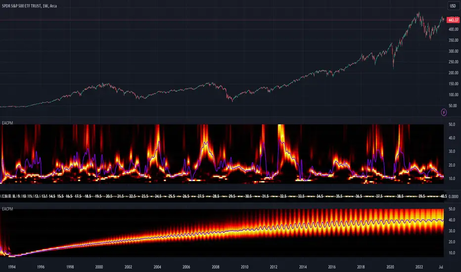
PERIODOGRAM INTERPRETATION:
The periodogram renders the power spectrum of a signal, with the y-axis representing the periodicity (frequencies/wavelengths) and the x-axis representing time. The y-axis is divided into periods, with each elevation representing a period. In this periodogram, the y-axis ranges from 6 at the very bottom to 49 at the top, with intermediate values in between, all indicating the power of the corresponding frequency component by color. The higher the position occurs on the y-axis, the longer the period or lower the frequency. The x-axis of the periodogram represents time and is divided into equal intervals, with each vertical column on the axis corresponding to the time interval when the signal was measured. The most recent values/colors are on the right side.
The intensity of the colors on the periodogram indicate the power level of the corresponding frequency or period. The fire color scheme is distinctly like the heat intensity from any casual flame witnessed in a small fire from a lighter, match, or camp fire. The most intense power would be indicated by the brightest of yellow, while the lowest power would be indicated by the darkest shade of red or just black. By analyzing the pattern of colors across different periods, one may gain insights into the dominant frequency components of the signal and visually identify recurring cycles/patterns of periodicity.
SETTINGS CONFIGURATIONS BRIEFLY EXPLAINED:
Source Options: These settings allow you to choose the data source for the analysis. Using the `Source` selection, you may tether to additional data streams (e.g. close, hlcc4, hl2), which also may include samples from any other indicator. For example, this could be my "Chirped Sine Wave Generator" script found in my member profile. By using the `SineWave` selection, you may analyze a theoretical sinusoidal wave with a user-defined period, something already incorporated into the code. The `SineWave` will be displayed over top of the periodogram.
Roofing Filter Options: These inputs control the range of the passband for ACP to analyze. Ehlers had two versions of his highpass filters for his releases, so I included an option for you to see the obvious difference when performing a comparison of both. You may choose between 1st and 2nd order high-pass filters.
Spectral Controls: These settings control the core functionality of the spectral analysis results. You can adjust the autocorrelation lag, adjust the level of smoothing for Fourier coefficients, and control the contrast/behavior of the heatmap displaying the power spectra. I provided two color schemes by checking or unchecking a checkbox.
Dominant Cycle Options: These settings allow you to customize the various types of dominant cycle values. You can choose between floating-point and integer values, and select the rounding method used to derive the final dominantCycle values. Also, you may control the level of smoothing applied to the dominant cycle values.
DOMINANT CYCLE VALUE SELECTIONS:
External to the acs() function, the code takes a dominant cycle value returned from acs() and changes its numeric form based on a specified type and form chosen within the indicator settings. The dominant cycle value can be represented as an integer or a decimal number, depending on the attached algorithm's requirements. For example, FIR filters will require an integer while many IIR filters can use a float. The float forms can be either rounded, smoothed, or floored. If the resulting value is desired to be an integer, it can be rounded up/down or just be in an integer form, depending on how your algorithm may utilize it.
AUTOCORRELATION SPECTRUM FUNCTION BASICALLY EXPLAINED:
In the beginning of the acs() code, the population of caches for precalculated angular frequency factors and smoothing coefficients occur. By precalculating these factors/coefs only once and then storing them in an array, the indicator can save time and computational resources when performing subsequent calculations that require them later.
In the following code block, the "Calculate AutoCorrelations" is calculated for each period within the passband width. The calculation involves numerous summations of values extracted from the roofing filter. Finally, a correlation values array is populated with the resulting values, which are normalized correlation coefficients.
Moving on to the next block of code, labeled "Decompose Fourier Components", Fourier decomposition is performed on the autocorrelation coefficients. It iterates this time through the applicable period range of 6 to 49, calculating the real and imaginary parts of the Fourier components. Frequencies 6 to 49 are the primary focus of interest for this periodogram. Using the precalculated angular frequency factors, the resulting real and imaginary parts are then utilized to calculate the spectral Fourier components, which are stored in an array for later use.
The next section of code smooths the noise ridden Fourier components between the periods of 6 and 49 with a selected filter. This species also employs numerous SuperSmoothers to condition noisy Fourier components. One of the big differences is Ehlers' versions used basic EMAs in this section of code. I decided to add SuperSmoothers.
The final sections of the acs() code determines the peak power component for normalization and then computes the dominant cycle period from the smoothed Fourier components. It first identifies a single spectral component with the highest power value and then assigns it as the peak power. Next, it normalizes the spectral components using the peak power value as a denominator. It then calculates the average dominant cycle period from the normalized spectral components using Ehlers' "Center of Gravity" calculation. Finally, the function returns the dominant cycle period along with the normalized spectral components for later external use to plot the periodogram.
POST SCRIPT:
Concluding, I have to acknowledge a newly found analyst for assistance that I couldn't receive from anywhere else. For one, Claude doesn't know much about Pine, is unfortunately color blind, and can't even see the Pine reference, but it was able to intuitively shred my code with laser precise realizations. Not only that, formulating and reformulating my description needed crucial finesse applied to it, and I couldn't have provided what you have read here without that artificial insight. Finding the right order of words to convey the complexity of ACP and the elaborate accompanying content was a daunting task. No code in my life has ever absorbed so much time and hard fricking work, than what you witness here, an ACP gem cut pristinely. I'm unveiling my version of ACP for an empowering cause, in the hopes a future global army of code wielders will tether it to highly functional computational contraptions they might possess. Here is ACP fully blessed poetically with the "Power of Pine" in sublime code. ENJOY!
GKD-M Baseline Optimizer [Loxx]Giga Kaleidoscope GKD-M Baseline Optimizer is a Metamorphosis module included in Loxx's "Giga Kaleidoscope Modularized Trading System".
The Baseline Optimizer enables traders to backtest over 60 moving averages using variable period inputs. It then exports the baseline with the highest cumulative win rate per candle to any baseline-enabled GKD backtest. To perform the backtesting, the trader selects an initial period input (default is 60) and a skip value that increments the initial period input up to seven times. For instance, if a skip value of 5 is chosen, the Baseline Optimizer will run the backtest for the selected moving average on periods such as 60, 65, 70, 75, and so on, up to 90. If the user selects an initial period input of 45 and a skip value of 2, the Baseline Optimizer will conduct backtests for the chosen moving average on periods like 45, 47, 49, 51, and so forth, up to 57.
The Baseline Optimizer provides a table displaying the output of the backtests for a specified date range. The table output represents the cumulative win rate for the given date range.
On the Metamorphosis side of the Baseline Optimizer, a cumulative backtest is calculated for each candle within the date range. This means that each candle may exhibit a different distribution of period inputs with the highest win rate for a particular moving average. The Baseline Optimizer identifies the period input combination with the highest win rates for long and short positions and creates a win-rate adaptive long and short moving average chart. The moving average used for shorts differs from the moving average used for longs, and the moving average for each candle may vary from any other candle. This customized baseline can then be exported to all baseline-enabled GKD backtests.
The backtest employed in the Baseline Optimizer is a Solo Confirmation Simple, allowing only one take profit and one stop loss to be set.
Lastly, the Baseline Optimizer incorporates Goldie Locks Zone filtering, which can be utilized for signal generation in advanced GKD backtests.
█ Moving Averages included in the Baseline Optimizer
Adaptive Moving Average - AMA
ADXvma - Average Directional Volatility Moving Average
Ahrens Moving Average
Alexander Moving Average - ALXMA
Deviation Scaled Moving Average - DSMA
Donchian
Double Exponential Moving Average - DEMA
Double Smoothed Exponential Moving Average - DSEMA
Double Smoothed FEMA - DSFEMA
Double Smoothed Range Weighted EMA - DSRWEMA
Double Smoothed Wilders EMA - DSWEMA
Double Weighted Moving Average - DWMA
Exponential Moving Average - EMA
Fast Exponential Moving Average - FEMA
Fractal Adaptive Moving Average - FRAMA
Generalized DEMA - GDEMA
Generalized Double DEMA - GDDEMA
Hull Moving Average (Type 1) - HMA1
Hull Moving Average (Type 2) - HMA2
Hull Moving Average (Type 3) - HMA3
Hull Moving Average (Type 4) - HMA4
IE /2 - Early T3 by Tim Tilson
Integral of Linear Regression Slope - ILRS
Kaufman Adaptive Moving Average - KAMA
Leader Exponential Moving Average
Linear Regression Value - LSMA ( Least Squares Moving Average )
Linear Weighted Moving Average - LWMA
McGinley Dynamic
McNicholl EMA
Non-Lag Moving Average
Ocean NMA Moving Average - ONMAMA
One More Moving Average - OMA
Parabolic Weighted Moving Average
Probability Density Function Moving Average - PDFMA
Quadratic Regression Moving Average - QRMA
Regularized EMA - REMA
Range Weighted EMA - RWEMA
Recursive Moving Trendline
Simple Decycler - SDEC
Simple Jurik Moving Average - SJMA
Simple Moving Average - SMA
Sine Weighted Moving Average
Smoothed LWMA - SLWMA
Smoothed Moving Average - SMMA
Smoother
Super Smoother
T3
Three-pole Ehlers Butterworth
Three-pole Ehlers Smoother
Triangular Moving Average - TMA
Triple Exponential Moving Average - TEMA
Two-pole Ehlers Butterworth
Two-pole Ehlers smoother
Variable Index Dynamic Average - VIDYA
Variable Moving Average - VMA
Volume Weighted EMA - VEMA
Volume Weighted Moving Average - VWMA
Zero-Lag DEMA - Zero Lag Exponential Moving Average
Zero-Lag Moving Average
Zero Lag TEMA - Zero Lag Triple Exponential Moving Average
Adaptive Moving Average - AMA
The Adaptive Moving Average (AMA) is a moving average that changes its sensitivity to price moves depending on the calculated volatility. It becomes more sensitive during periods when the price is moving smoothly in a certain direction and becomes less sensitive when the price is volatile.
ADXvma - Average Directional Volatility Moving Average
Linnsoft's ADXvma formula is a volatility-based moving average, with the volatility being determined by the value of the ADX indicator.
The ADXvma has the SMA in Chande's CMO replaced with an EMA , it then uses a few more layers of EMA smoothing before the "Volatility Index" is calculated.
A side effect is, those additional layers slow down the ADXvma when you compare it to Chande's Variable Index Dynamic Average VIDYA .
The ADXVMA provides support during uptrends and resistance during downtrends and will stay flat for longer, but will create some of the most accurate market signals when it decides to move.
Ahrens Moving Average
Richard D. Ahrens's Moving Average promises "Smoother Data" that isn't influenced by the occasional price spike. It works by using the Open and the Close in his formula so that the only time the Ahrens Moving Average will change is when the candlestick is either making new highs or new lows.
Alexander Moving Average - ALXMA
This Moving Average uses an elaborate smoothing formula and utilizes a 7 period Moving Average. It corresponds to fitting a second-order polynomial to seven consecutive observations. This moving average is rarely used in trading but is interesting as this Moving Average has been applied to diffusion indexes that tend to be very volatile.
Deviation Scaled Moving Average - DSMA
The Deviation-Scaled Moving Average is a data smoothing technique that acts like an exponential moving average with a dynamic smoothing coefficient. The smoothing coefficient is automatically updated based on the magnitude of price changes. In the Deviation-Scaled Moving Average, the standard deviation from the mean is chosen to be the measure of this magnitude. The resulting indicator provides substantial smoothing of the data even when price changes are small while quickly adapting to these changes.
Donchian
Donchian Channels are three lines generated by moving average calculations that comprise an indicator formed by upper and lower bands around a midrange or median band. The upper band marks the highest price of a security over N periods while the lower band marks the lowest price of a security over N periods.
Double Exponential Moving Average - DEMA
The Double Exponential Moving Average ( DEMA ) combines a smoothed EMA and a single EMA to provide a low-lag indicator. It's primary purpose is to reduce the amount of "lagging entry" opportunities, and like all Moving Averages, the DEMA confirms uptrends whenever price crosses on top of it and closes above it, and confirms downtrends when the price crosses under it and closes below it - but with significantly less lag.
Double Smoothed Exponential Moving Average - DSEMA
The Double Smoothed Exponential Moving Average is a lot less laggy compared to a traditional EMA . It's also considered a leading indicator compared to the EMA , and is best utilized whenever smoothness and speed of reaction to market changes are required.
Double Smoothed FEMA - DSFEMA
Same as the Double Exponential Moving Average (DEMA), but uses a faster version of EMA for its calculation.
Double Smoothed Range Weighted EMA - DSRWEMA
Range weighted exponential moving average (EMA) is, unlike the "regular" range weighted average calculated in a different way. Even though the basis - the range weighting - is the same, the way how it is calculated is completely different. By definition this type of EMA is calculated as a ratio of EMA of price*weight / EMA of weight. And the results are very different and the two should be considered as completely different types of averages. The higher than EMA to price changes responsiveness when the ranges increase remains in this EMA too and in those cases this EMA is clearly leading the "regular" EMA. This version includes double smoothing.
Double Smoothed Wilders EMA - DSWEMA
Welles Wilder was frequently using one "special" case of EMA (Exponential Moving Average) that is due to that fact (that he used it) sometimes called Wilder's EMA. This version is adding double smoothing to Wilder's EMA in order to make it "faster" (it is more responsive to market prices than the original) and is still keeping very smooth values.
Double Weighted Moving Average - DWMA
Double weighted moving average is an LWMA (Linear Weighted Moving Average). Instead of doing one cycle for calculating the LWMA, the indicator is made to cycle the loop 2 times. That produces a smoother values than the original LWMA
Exponential Moving Average - EMA
The EMA places more significance on recent data points and moves closer to price than the SMA ( Simple Moving Average ). It reacts faster to volatility due to its emphasis on recent data and is known for its ability to give greater weight to recent and more relevant data. The EMA is therefore seen as an enhancement over the SMA .
Fast Exponential Moving Average - FEMA
An Exponential Moving Average with a short look-back period.
Fractal Adaptive Moving Average - FRAMA
The Fractal Adaptive Moving Average by John Ehlers is an intelligent adaptive Moving Average which takes the importance of price changes into account and follows price closely enough to display significant moves whilst remaining flat if price ranges. The FRAMA does this by dynamically adjusting the look-back period based on the market's fractal geometry.
Generalized DEMA - GDEMA
The double exponential moving average (DEMA), was developed by Patrick Mulloy in an attempt to reduce the amount of lag time found in traditional moving averages. It was first introduced in the February 1994 issue of the magazine Technical Analysis of Stocks & Commodities in Mulloy's article "Smoothing Data with Faster Moving Averages.". Instead of using fixed multiplication factor in the final DEMA formula, the generalized version allows you to change it. By varying the "volume factor" form 0 to 1 you apply different multiplications and thus producing DEMA with different "speed" - the higher the volume factor is the "faster" the DEMA will be (but also the slope of it will be less smooth). The volume factor is limited in the calculation to 1 since any volume factor that is larger than 1 is increasing the overshooting to the extent that some volume factors usage makes the indicator unusable.
Generalized Double DEMA - GDDEMA
The double exponential moving average (DEMA), was developed by Patrick Mulloy in an attempt to reduce the amount of lag time found in traditional moving averages. It was first introduced in the February 1994 issue of the magazine Technical Analysis of Stocks & Commodities in Mulloy's article "Smoothing Data with Faster Moving Averages''. This is an extension of the Generalized DEMA using Tim Tillsons (the inventor of T3) idea, and is using GDEMA of GDEMA for calculation (which is the "middle step" of T3 calculation). Since there are no versions showing that middle step, this version covers that too. The result is smoother than Generalized DEMA, but is less smooth than T3 - one has to do some experimenting in order to find the optimal way to use it, but in any case, since it is "faster" than the T3 (Tim Tillson T3) and still smooth, it looks like a good compromise between speed and smoothness.
Hull Moving Average (Type 1) - HMA1
Alan Hull's HMA makes use of weighted moving averages to prioritize recent values and greatly reduce lag whilst maintaining the smoothness of a traditional Moving Average. For this reason, it's seen as a well-suited Moving Average for identifying entry points. This version uses SMA for smoothing.
Hull Moving Average (Type 2) - HMA2
Alan Hull's HMA makes use of weighted moving averages to prioritize recent values and greatly reduce lag whilst maintaining the smoothness of a traditional Moving Average. For this reason, it's seen as a well-suited Moving Average for identifying entry points. This version uses EMA for smoothing.
Hull Moving Average (Type 3) - HMA3
Alan Hull's HMA makes use of weighted moving averages to prioritize recent values and greatly reduce lag whilst maintaining the smoothness of a traditional Moving Average. For this reason, it's seen as a well-suited Moving Average for identifying entry points. This version uses LWMA for smoothing.
Hull Moving Average (Type 4) - HMA4
Alan Hull's HMA makes use of weighted moving averages to prioritize recent values and greatly reduce lag whilst maintaining the smoothness of a traditional Moving Average. For this reason, it's seen as a well-suited Moving Average for identifying entry points. This version uses SMMA for smoothing.
IE /2 - Early T3 by Tim Tilson and T3 new
The T3 moving average is a type of technical indicator used in financial analysis to identify trends in price movements. It is similar to the Exponential Moving Average (EMA) and the Double Exponential Moving Average (DEMA), but uses a different smoothing algorithm.
The T3 moving average is calculated using a series of exponential moving averages that are designed to filter out noise and smooth the data. The resulting smoothed data is then weighted with a non-linear function to produce a final output that is more responsive to changes in trend direction.
The T3 moving average can be customized by adjusting the length of the moving average, as well as the weighting function used to smooth the data. It is commonly used in conjunction with other technical indicators as part of a larger trading strategy.
Integral of Linear Regression Slope - ILRS
A Moving Average where the slope of a linear regression line is simply integrated as it is fitted in a moving window of length N (natural numbers in maths) across the data. The derivative of ILRS is the linear regression slope. ILRS is not the same as a SMA ( Simple Moving Average ) of length N, which is actually the midpoint of the linear regression line as it moves across the data.
Kaufman Adaptive Moving Average - KAMA
Developed by Perry Kaufman, Kaufman's Adaptive Moving Average (KAMA) is a moving average designed to account for market noise or volatility. KAMA will closely follow prices when the price swings are relatively small and the noise is low.
Leader Exponential Moving Average
The Leader EMA was created by Giorgos E. Siligardos who created a Moving Average which was able to eliminate lag altogether whilst maintaining some smoothness. It was first described during his research paper "MACD Leader" where he applied this to the MACD to improve its signals and remove its lagging issue. This filter uses his leading MACD's "modified EMA" and can be used as a zero lag filter.
Linear Regression Value - LSMA ( Least Squares Moving Average )
LSMA as a Moving Average is based on plotting the end point of the linear regression line. It compares the current value to the prior value and a determination is made of a possible trend, eg. the linear regression line is pointing up or down.
Linear Weighted Moving Average - LWMA
LWMA reacts to price quicker than the SMA and EMA . Although it's similar to the Simple Moving Average , the difference is that a weight coefficient is multiplied to the price which means the most recent price has the highest weighting, and each prior price has progressively less weight. The weights drop in a linear fashion.
McGinley Dynamic
John McGinley created this Moving Average to track prices better than traditional Moving Averages. It does this by incorporating an automatic adjustment factor into its formula, which speeds (or slows) the indicator in trending, or ranging, markets.
McNicholl EMA
Dennis McNicholl developed this Moving Average to use as his center line for his "Better Bollinger Bands" indicator and was successful because it responded better to volatility changes over the standard SMA and managed to avoid common whipsaws.
Non-lag moving average
The Non Lag Moving average follows price closely and gives very quick signals as well as early signals of price change. As a standalone Moving Average, it should not be used on its own, but as an additional confluence tool for early signals.
Ocean NMA Moving Average - ONMAMA
Created by Jim Sloman, the NMA is a moving average that automatically adjusts to volatility without being programmed to do so. For more info, read his guide "Ocean Theory, an Introduction"
One More Moving Average (OMA)
The One More Moving Average (OMA) is a technical indicator that calculates a series of Jurik-style moving averages in order to reduce noise and provide smoother price data. It uses six exponential moving averages to generate the final value, with the length of the moving averages determined by an adaptive algorithm that adjusts to the current market conditions. The algorithm calculates the average period by comparing the signal to noise ratio and using this value to determine the length of the moving averages. The resulting values are used to generate the final value of the OMA, which can be used to identify trends and potential changes in trend direction.
Parabolic Weighted Moving Average
The Parabolic Weighted Moving Average is a variation of the Linear Weighted Moving Average . The Linear Weighted Moving Average calculates the average by assigning different weights to each element in its calculation. The Parabolic Weighted Moving Average is a variation that allows weights to be changed to form a parabolic curve. It is done simply by using the Power parameter of this indicator.
Probability Density Function Moving Average - PDFMA
Probability density function based MA is a sort of weighted moving average that uses probability density function to calculate the weights. By its nature it is similar to a lot of digital filters.
Quadratic Regression Moving Average - QRMA
A quadratic regression is the process of finding the equation of the parabola that best fits a set of data. This moving average is an obscure concept that was posted to Forex forums in around 2008.
Regularized EMA - REMA
The regularized exponential moving average (REMA) by Chris Satchwell is a variation on the EMA (see Exponential Moving Average) designed to be smoother but not introduce too much extra lag.
Range Weighted EMA - RWEMA
This indicator is a variation of the range weighted EMA. The variation comes from a possible need to make that indicator a bit less "noisy" when it comes to slope changes. The method used for calculating this variation is the method described by Lee Leibfarth in his article "Trading With An Adaptive Price Zone".
Recursive Moving Trendline
Dennis Meyers's Recursive Moving Trendline uses a recursive (repeated application of a rule) polynomial fit, a technique that uses a small number of past values estimations of price and today's price to predict tomorrow's price.
Simple Decycler - SDEC
The Ehlers Simple Decycler study is a virtually zero-lag technical indicator proposed by John F. Ehlers. The original idea behind this study (and several others created by John F. Ehlers) is that market data can be considered a continuum of cycle periods with different cycle amplitudes. Thus, trending periods can be considered segments of longer cycles, or, in other words, low-frequency segments. Applying the right filter might help identify these segments.
Simple Loxx Moving Average - SLMA
A three stage moving average combining an adaptive EMA, a Kalman Filter, and a Kauffman adaptive filter.
Simple Moving Average - SMA
The SMA calculates the average of a range of prices by adding recent prices and then dividing that figure by the number of time periods in the calculation average. It is the most basic Moving Average which is seen as a reliable tool for starting off with Moving Average studies. As reliable as it may be, the basic moving average will work better when it's enhanced into an EMA .
Sine Weighted Moving Average
The Sine Weighted Moving Average assigns the most weight at the middle of the data set. It does this by weighting from the first half of a Sine Wave Cycle and the most weighting is given to the data in the middle of that data set. The Sine WMA closely resembles the TMA (Triangular Moving Average).
Smoothed LWMA - SLWMA
A smoothed version of the LWMA
Smoothed Moving Average - SMMA
The Smoothed Moving Average is similar to the Simple Moving Average ( SMA ), but aims to reduce noise rather than reduce lag. SMMA takes all prices into account and uses a long lookback period. Due to this, it's seen as an accurate yet laggy Moving Average.
Smoother
The Smoother filter is a faster-reacting smoothing technique which generates considerably less lag than the SMMA ( Smoothed Moving Average ). It gives earlier signals but can also create false signals due to its earlier reactions. This filter is sometimes wrongly mistaken for the superior Jurik Smoothing algorithm.
Super Smoother
The Super Smoother filter uses John Ehlers’s “Super Smoother” which consists of a Two pole Butterworth filter combined with a 2-bar SMA ( Simple Moving Average ) that suppresses the 22050 Hz Nyquist frequency: A characteristic of a sampler, which converts a continuous function or signal into a discrete sequence.
Three-pole Ehlers Butterworth
The 3 pole Ehlers Butterworth (as well as the Two pole Butterworth) are both superior alternatives to the EMA and SMA . They aim at producing less lag whilst maintaining accuracy. The 2 pole filter will give you a better approximation for price, whereas the 3 pole filter has superior smoothing.
Three-pole Ehlers smoother
The 3 pole Ehlers smoother works almost as close to price as the above mentioned 3 Pole Ehlers Butterworth. It acts as a strong baseline for signals but removes some noise. Side by side, it hardly differs from the Three Pole Ehlers Butterworth but when examined closely, it has better overshoot reduction compared to the 3 pole Ehlers Butterworth.
Triangular Moving Average - TMA
The TMA is similar to the EMA but uses a different weighting scheme. Exponential and weighted Moving Averages will assign weight to the most recent price data. Simple moving averages will assign the weight equally across all the price data. With a TMA (Triangular Moving Average), it is double smoother (averaged twice) so the majority of the weight is assigned to the middle portion of the data.
Triple Exponential Moving Average - TEMA
The TEMA uses multiple EMA calculations as well as subtracting lag to create a tool which can be used for scalping pullbacks. As it follows price closely, its signals are considered very noisy and should only be used in extremely fast-paced trading conditions.
Two-pole Ehlers Butterworth
The 2 pole Ehlers Butterworth (as well as the three pole Butterworth mentioned above) is another filter that cuts out the noise and follows the price closely. The 2 pole is seen as a faster, leading filter over the 3 pole and follows price a bit more closely. Analysts will utilize both a 2 pole and a 3 pole Butterworth on the same chart using the same period, but having both on chart allows its crosses to be traded.
Two-pole Ehlers smoother
A smoother version of the Two pole Ehlers Butterworth. This filter is the faster version out of the 3 pole Ehlers Butterworth. It does a decent job at cutting out market noise whilst emphasizing a closer following to price over the 3 pole Ehlers .
Variable Index Dynamic Average - VIDYA
Variable Index Dynamic Average Technical Indicator ( VIDYA ) was developed by Tushar Chande. It is an original method of calculating the Exponential Moving Average ( EMA ) with the dynamically changing period of averaging.
Variable Moving Average - VMA
The Variable Moving Average (VMA) is a study that uses an Exponential Moving Average being able to automatically adjust its smoothing factor according to the market volatility.
Volume Weighted EMA - VEMA
An EMA that uses a volume and price weighted calculation instead of the standard price input.
Volume Weighted Moving Average - VWMA
A Volume Weighted Moving Average is a moving average where more weight is given to bars with heavy volume than with light volume. Thus the value of the moving average will be closer to where most trading actually happened than it otherwise would be without being volume weighted.
Zero-Lag DEMA - Zero Lag Double Exponential Moving Average
John Ehlers's Zero Lag DEMA's aim is to eliminate the inherent lag associated with all trend following indicators which average a price over time. Because this is a Double Exponential Moving Average with Zero Lag, it has a tendency to overshoot and create a lot of false signals for swing trading. It can however be used for quick scalping or as a secondary indicator for confluence.
Zero-Lag Moving Average
The Zero Lag Moving Average is described by its creator, John Ehlers , as a Moving Average with absolutely no delay. And it's for this reason that this filter will cause a lot of abrupt signals which will not be ideal for medium to long-term traders. This filter is designed to follow price as close as possible whilst de-lagging data instead of basing it on regular data. The way this is done is by attempting to remove the cumulative effect of the Moving Average.
Zero-Lag TEMA - Zero Lag Triple Exponential Moving Average
Just like the Zero Lag DEMA , this filter will give you the fastest signals out of all the Zero Lag Moving Averages. This is useful for scalping but dangerous for medium to long-term traders, especially during market Volatility and news events. Having no lag, this filter also has no smoothing in its signals and can cause some very bizarre behavior when applied to certain indicators.
█ Volatility Goldie Locks Zone
The Goldie Locks Zone volatility filter is the standard first-pass filter used in all advanced GKD backtests (Complex, Super Complex, and Full GKd). This filter requires the price to fall within a range determined by multiples of volatility. The Goldie Locks Zone is separate from the core Baseline and utilizes its own moving average with Loxx's Exotic Source Types you can read about below.
On the chart, you will find green and red dots positioned at the top, indicating whether a candle qualifies for a long or short trade respectively. Additionally, green and red triangles are located at the bottom of the chart, signifying whether the trigger has crossed up or down and qualifies within the Goldie Locks zone. The Goldie Locks zone is represented by a white color on the mean line, indicating low volatility levels that are not suitable for trading.
█ Volatility Types Included in the Baseline Optimizer
The GKD system utilizes volatility-based take profits and stop losses. Each take profit and stop loss is calculated as a multiple of volatility. Users can also adjust the multiplier values in the settings.
This module includes 17 types of volatility:
Close-to-Close
Parkinson
Garman-Klass
Rogers-Satchell
Yang-Zhang
Garman-Klass-Yang-Zhang
Exponential Weighted Moving Average
Standard Deviation of Log Returns
Pseudo GARCH(2,2)
Average True Range
True Range Double
Standard Deviation
Adaptive Deviation
Median Absolute Deviation
Efficiency-Ratio Adaptive ATR
Mean Absolute Deviation
Static Percent
Various volatility estimators and indicators that investors and traders can use to measure the dispersion or volatility of a financial instrument's price. Each estimator has its strengths and weaknesses, and the choice of estimator should depend on the specific needs and circumstances of the user.
Close-to-Close
Close-to-Close volatility is a classic and widely used volatility measure, sometimes referred to as historical volatility.
Volatility is an indicator of the speed of a stock price change. A stock with high volatility is one where the price changes rapidly and with a larger amplitude. The more volatile a stock is, the riskier it is.
Close-to-close historical volatility is calculated using only a stock's closing prices. It is the simplest volatility estimator. However, in many cases, it is not precise enough. Stock prices could jump significantly during a trading session and return to the opening value at the end. That means that a considerable amount of price information is not taken into account by close-to-close volatility.
Despite its drawbacks, Close-to-Close volatility is still useful in cases where the instrument doesn't have intraday prices. For example, mutual funds calculate their net asset values daily or weekly, and thus their prices are not suitable for more sophisticated volatility estimators.
Parkinson
Parkinson volatility is a volatility measure that uses the stock’s high and low price of the day.
The main difference between regular volatility and Parkinson volatility is that the latter uses high and low prices for a day, rather than only the closing price. This is useful as close-to-close prices could show little difference while large price movements could have occurred during the day. Thus, Parkinson's volatility is considered more precise and requires less data for calculation than close-to-close volatility.
One drawback of this estimator is that it doesn't take into account price movements after the market closes. Hence, it systematically undervalues volatility. This drawback is addressed in the Garman-Klass volatility estimator.
Garman-Klass
Garman-Klass is a volatility estimator that incorporates open, low, high, and close prices of a security.
Garman-Klass volatility extends Parkinson's volatility by taking into account the opening and closing prices. As markets are most active during the opening and closing of a trading session, it makes volatility estimation more accurate.
Garman and Klass also assumed that the process of price change follows a continuous diffusion process (Geometric Brownian motion). However, this assumption has several drawbacks. The method is not robust for opening jumps in price and trend movements.
Despite its drawbacks, the Garman-Klass estimator is still more effective than the basic formula since it takes into account not only the price at the beginning and end of the time interval but also intraday price extremes.
Researchers Rogers and Satchell have proposed a more efficient method for assessing historical volatility that takes into account price trends. See Rogers-Satchell Volatility for more detail.
Rogers-Satchell
Rogers-Satchell is an estimator for measuring the volatility of securities with an average return not equal to zero.
Unlike Parkinson and Garman-Klass estimators, Rogers-Satchell incorporates a drift term (mean return not equal to zero). As a result, it provides better volatility estimation when the underlying is trending.
The main disadvantage of this method is that it does not take into account price movements between trading sessions. This leads to an underestimation of volatility since price jumps periodically occur in the market precisely at the moments between sessions.
A more comprehensive estimator that also considers the gaps between sessions was developed based on the Rogers-Satchel formula in the 2000s by Yang-Zhang. See Yang Zhang Volatility for more detail.
Yang-Zhang
Yang Zhang is a historical volatility estimator that handles both opening jumps and the drift and has a minimum estimation error.
Yang-Zhang volatility can be thought of as a combination of the overnight (close-to-open volatility) and a weighted average of the Rogers-Satchell volatility and the day’s open-to-close volatility. It is considered to be 14 times more efficient than the close-to-close estimator.
Garman-Klass-Yang-Zhang
Garman-Klass-Yang-Zhang (GKYZ) volatility estimator incorporates the returns of open, high, low, and closing prices in its calculation.
GKYZ volatility estimator takes into account overnight jumps but not the trend, i.e., it assumes that the underlying asset follows a Geometric Brownian Motion (GBM) process with zero drift. Therefore, the GKYZ volatility estimator tends to overestimate the volatility when the drift is different from zero. However, for a GBM process, this estimator is eight times more efficient than the close-to-close volatility estimator.
Exponential Weighted Moving Average
The Exponentially Weighted Moving Average (EWMA) is a quantitative or statistical measure used to model or describe a time series. The EWMA is widely used in finance, with the main applications being technical analysis and volatility modeling.
The moving average is designed such that older observations are given lower weights. The weights decrease exponentially as the data point gets older – hence the name exponentially weighted.
The only decision a user of the EWMA must make is the parameter lambda. The parameter decides how important the current observation is in the calculation of the EWMA. The higher the value of lambda, the more closely the EWMA tracks the original time series.
Standard Deviation of Log Returns
This is the simplest calculation of volatility. It's the standard deviation of ln(close/close(1)).
Pseudo GARCH(2,2)
This is calculated using a short- and long-run mean of variance multiplied by ?.
?avg(var;M) + (1 ? ?) avg(var;N) = 2?var/(M+1-(M-1)L) + 2(1-?)var/(M+1-(M-1)L)
Solving for ? can be done by minimizing the mean squared error of estimation; that is, regressing L^-1var - avg(var; N) against avg(var; M) - avg(var; N) and using the resulting beta estimate as ?.
Average True Range
The average true range (ATR) is a technical analysis indicator, introduced by market technician J. Welles Wilder Jr. in his book New Concepts in Technical Trading Systems, that measures market volatility by decomposing the entire range of an asset price for that period.
The true range indicator is taken as the greatest of the following: current high less the current low; the absolute value of the current high less the previous close; and the absolute value of the current low less the previous close. The ATR is then a moving average, generally using 14 days, of the true ranges.
True Range Double
A special case of ATR that attempts to correct for volatility skew.
Standard Deviation
Standard deviation is a statistic that measures the dispersion of a dataset relative to its mean and is calculated as the square root of the variance. The standard deviation is calculated as the square root of variance by determining each data point's deviation relative to the mean. If the data points are further from the mean, there is a higher deviation within the data set; thus, the more spread out the data, the higher the standard deviation.
Adaptive Deviation
By definition, the Standard Deviation (STD, also represented by the Greek letter sigma ? or the Latin letter s) is a measure that is used to quantify the amount of variation or dispersion of a set of data values. In technical analysis, we usually use it to measure the level of current volatility.
Standard Deviation is based on Simple Moving Average calculation for mean value. This version of standard deviation uses the properties of EMA to calculate what can be called a new type of deviation, and since it is based on EMA, we can call it EMA deviation. Additionally, Perry Kaufman's efficiency ratio is used to make it adaptive (since all EMA type calculations are nearly perfect for adapting).
The difference when compared to the standard is significant--not just because of EMA usage, but the efficiency ratio makes it a "bit more logical" in very volatile market conditions.
Median Absolute Deviation
The median absolute deviation is a measure of statistical dispersion. Moreover, the MAD is a robust statistic, being more resilient to outliers in a data set than the standard deviation. In the standard deviation, the distances from the mean are squared, so large deviations are weighted more heavily, and thus outliers can heavily influence it. In the MAD, the deviations of a small number of outliers are irrelevant.
Because the MAD is a more robust estimator of scale than the sample variance or standard deviation, it works better with distributions without a mean or variance, such as the Cauchy distribution.
For this indicator, a manual recreation of the quantile function in Pine Script is used. This is so users have a full inside view into how this is calculated.
Efficiency-Ratio Adaptive ATR
Average True Range (ATR) is a widely used indicator for many occasions in technical analysis. It is calculated as the RMA of the true range. This version adds a "twist": it uses Perry Kaufman's Efficiency Ratio to calculate adaptive true range.
Mean Absolute Deviation
The mean absolute deviation (MAD) is a measure of variability that indicates the average distance between observations and their mean. MAD uses the original units of the data, which simplifies interpretation. Larger values signify that the data points spread out further from the average. Conversely, lower values correspond to data points bunching closer to it. The mean absolute deviation is also known as the mean deviation and average absolute deviation.
This definition of the mean absolute deviation sounds similar to the standard deviation (SD). While both measure variability, they have different calculations. In recent years, some proponents of MAD have suggested that it replace the SD as the primary measure because it is a simpler concept that better fits real life.
█ Loxx's Expanded Source Types Included in Baseline Optimizer
This indicator allows you to select from 33 source types. They are as follows:
Close
Open
High
Low
Median
Typical
Weighted
Average
Average Median Body
Trend Biased
Trend Biased (Extreme)
HA Close
HA Open
HA High
HA Low
HA Median
HA Typical
HA Weighted
HA Average
HA Average Median Body
HA Trend Biased
HA Trend Biased (Extreme)
HAB Close
HAB Open
HAB High
HAB Low
HAB Median
HAB Typical
HAB Weighted
HAB Average
HAB Average Median Body
HAB Trend Biased
HAB Trend Biased (Extreme)
What are Heiken Ashi "better" candles?
Heiken Ashi "better" candles are a modified version of the standard Heiken Ashi candles, which are a popular charting technique used in technical analysis. Heiken Ashi candles help traders identify trends and potential reversal points by smoothing out price data and reducing market noise. The "better formula" was proposed by Sebastian Schmidt in an article published by BNP Paribas in Warrants & Zertifikate, a German magazine, in August 2004. The aim of this formula is to further improve the smoothing of the Heiken Ashi chart and enhance its effectiveness in identifying trends and reversals.
Standard Heiken Ashi candles are calculated using the following formulas:
Heiken Ashi Close = (Open + High + Low + Close) / 4
Heiken Ashi Open = (Previous Heiken Ashi Open + Previous Heiken Ashi Close) / 2
Heiken Ashi High = Max (High, Heiken Ashi Open, Heiken Ashi Close)
Heiken Ashi Low = Min (Low, Heiken Ashi Open, Heiken Ashi Close)
The "better formula" modifies the standard Heiken Ashi calculation by incorporating additional smoothing, which can help reduce noise and make it easier to identify trends and reversals. The modified formulas for Heiken Ashi "better" candles are as follows:
Better Heiken Ashi Close = (Open + High + Low + Close) / 4
Better Heiken Ashi Open = (Previous Better Heiken Ashi Open + Previous Better Heiken Ashi Close) / 2
Better Heiken Ashi High = Max (High, Better Heiken Ashi Open, Better Heiken Ashi Close)
Better Heiken Ashi Low = Min (Low, Better Heiken Ashi Open, Better Heiken Ashi Close)
Smoothing Factor = 2 / (N + 1), where N is the chosen period for smoothing
Smoothed Better Heiken Ashi Open = (Better Heiken Ashi Open * Smoothing Factor) + (Previous Smoothed Better Heiken Ashi Open * (1 - Smoothing Factor))
Smoothed Better Heiken Ashi Close = (Better Heiken Ashi Close * Smoothing Factor) + (Previous Smoothed Better Heiken Ashi Close * (1 - Smoothing Factor))
The smoothed Better Heiken Ashi Open and Close values are then used to calculate the smoothed Better Heiken Ashi High and Low values, resulting in "better" candles that provide a clearer representation of the market trend and potential reversal points.
Heiken Ashi "better" candles, as mentioned previously, provide a clearer representation of market trends and potential reversal points by reducing noise and smoothing out price data. When using these candles in conjunction with other technical analysis tools and indicators, traders can gain valuable insights into market behavior and make more informed decisions.
To effectively use Heiken Ashi "better" candles in your trading strategy, consider the following tips:
-Trend Identification: Heiken Ashi "better" candles can help you identify the prevailing trend in the market. When the majority of the candles are green (or another color, depending on your chart settings) and there are no or few lower wicks, it may indicate a strong uptrend. Conversely, when the majority of the candles are red (or another color) and there are no or few upper wicks, it may signal a strong downtrend.
-Trend Reversals: Look for potential trend reversals when a change in the color of the candles occurs, especially when accompanied by longer wicks. For example, if a green candle with a long lower wick is followed by a red candle, it could indicate a bearish reversal. Similarly, a red candle with a long upper wick followed by a green candle may suggest a bullish reversal.
-Support and Resistance: You can use Heiken Ashi "better" candles to identify potential support and resistance levels. When the candles are consistently moving in one direction and then suddenly change color with longer wicks, it could indicate the presence of a support or resistance level.
-Stop-Loss and Take-Profit: Using Heiken Ashi "better" candles can help you manage risk by determining optimal stop-loss and take-profit levels. For instance, you can place your stop-loss below the low of the most recent green candle in an uptrend or above the high of the most recent red candle in a downtrend.
-Confirming Signals: Heiken Ashi "better" candles should be used in conjunction with other technical indicators, such as moving averages, oscillators, or chart patterns, to confirm signals and improve the accuracy of your analysis.
In this implementation, you have the choice of AMA, KAMA, or T3 smoothing. These are as follows:
Kaufman Adaptive Moving Average (KAMA)
The Kaufman Adaptive Moving Average (KAMA) is a type of adaptive moving average used in technical analysis to smooth out price fluctuations and identify trends. The KAMA adjusts its smoothing factor based on the market's volatility, making it more responsive in volatile markets and smoother in calm markets. The KAMA is calculated using three different efficiency ratios that determine the appropriate smoothing factor for the current market conditions. These ratios are based on the noise level of the market, the speed at which the market is moving, and the length of the moving average. The KAMA is a popular choice among traders who prefer to use adaptive indicators to identify trends and potential reversals.
Adaptive Moving Average
The Adaptive Moving Average (AMA) is a type of moving average that adjusts its sensitivity to price movements based on market conditions. It uses a ratio between the current price and the highest and lowest prices over a certain lookback period to determine its level of smoothing. The AMA can help reduce lag and increase responsiveness to changes in trend direction, making it useful for traders who want to follow trends while avoiding false signals. The AMA is calculated by multiplying a smoothing constant with the difference between the current price and the previous AMA value, then adding the result to the previous AMA value.
T3
The T3 moving average is a type of technical indicator used in financial analysis to identify trends in price movements. It is similar to the Exponential Moving Average (EMA) and the Double Exponential Moving Average (DEMA), but uses a different smoothing algorithm.
The T3 moving average is calculated using a series of exponential moving averages that are designed to filter out noise and smooth the data. The resulting smoothed data is then weighted with a non-linear function to produce a final output that is more responsive to changes in trend direction.
The T3 moving average can be customized by adjusting the length of the moving average, as well as the weighting function used to smooth the data. It is commonly used in conjunction with other technical indicators as part of a larger trading strategy.
█ Giga Kaleidoscope Modularized Trading System
Core components of an NNFX algorithmic trading strategy
The NNFX algorithm is built on the principles of trend, momentum, and volatility. There are six core components in the NNFX trading algorithm:
1. Volatility - price volatility; e.g., Average True Range, True Range Double, Close-to-Close, etc.
2. Baseline - a moving average to identify price trend
3. Confirmation 1 - a technical indicator used to identify trends
4. Confirmation 2 - a technical indicator used to identify trends
5. Continuation - a technical indicator used to identify trends
6. Volatility/Volume - a technical indicator used to identify volatility/volume breakouts/breakdown
7. Exit - a technical indicator used to determine when a trend is exhausted
8. Metamorphosis - a technical indicator that produces a compound signal from the combination of other GKD indicators*
*(not part of the NNFX algorithm)
What is Volatility in the NNFX trading system?
In the NNFX (No Nonsense Forex) trading system, ATR (Average True Range) is typically used to measure the volatility of an asset. It is used as a part of the system to help determine the appropriate stop loss and take profit levels for a trade. ATR is calculated by taking the average of the true range values over a specified period.
True range is calculated as the maximum of the following values:
-Current high minus the current low
-Absolute value of the current high minus the previous close
-Absolute value of the current low minus the previous close
ATR is a dynamic indicator that changes with changes in volatility. As volatility increases, the value of ATR increases, and as volatility decreases, the value of ATR decreases. By using ATR in NNFX system, traders can adjust their stop loss and take profit levels according to the volatility of the asset being traded. This helps to ensure that the trade is given enough room to move, while also minimizing potential losses.
Other types of volatility include True Range Double (TRD), Close-to-Close, and Garman-Klass
What is a Baseline indicator?
The baseline is essentially a moving average, and is used to determine the overall direction of the market.
The baseline in the NNFX system is used to filter out trades that are not in line with the long-term trend of the market. The baseline is plotted on the chart along with other indicators, such as the Moving Average (MA), the Relative Strength Index (RSI), and the Average True Range (ATR).
Trades are only taken when the price is in the same direction as the baseline. For example, if the baseline is sloping upwards, only long trades are taken, and if the baseline is sloping downwards, only short trades are taken. This approach helps to ensure that trades are in line with the overall trend of the market, and reduces the risk of entering trades that are likely to fail.
By using a baseline in the NNFX system, traders can have a clear reference point for determining the overall trend of the market, and can make more informed trading decisions. The baseline helps to filter out noise and false signals, and ensures that trades are taken in the direction of the long-term trend.
What is a Confirmation indicator?
Confirmation indicators are technical indicators that are used to confirm the signals generated by primary indicators. Primary indicators are the core indicators used in the NNFX system, such as the Average True Range (ATR), the Moving Average (MA), and the Relative Strength Index (RSI).
The purpose of the confirmation indicators is to reduce false signals and improve the accuracy of the trading system. They are designed to confirm the signals generated by the primary indicators by providing additional information about the strength and direction of the trend.
Some examples of confirmation indicators that may be used in the NNFX system include the Bollinger Bands, the MACD (Moving Average Convergence Divergence), and the MACD Oscillator. These indicators can provide information about the volatility, momentum, and trend strength of the market, and can be used to confirm the signals generated by the primary indicators.
In the NNFX system, confirmation indicators are used in combination with primary indicators and other filters to create a trading system that is robust and reliable. By using multiple indicators to confirm trading signals, the system aims to reduce the risk of false signals and improve the overall profitability of the trades.
What is a Continuation indicator?
In the NNFX (No Nonsense Forex) trading system, a continuation indicator is a technical indicator that is used to confirm a current trend and predict that the trend is likely to continue in the same direction. A continuation indicator is typically used in conjunction with other indicators in the system, such as a baseline indicator, to provide a comprehensive trading strategy.
What is a Volatility/Volume indicator?
Volume indicators, such as the On Balance Volume (OBV), the Chaikin Money Flow (CMF), or the Volume Price Trend (VPT), are used to measure the amount of buying and selling activity in a market. They are based on the trading volume of the market, and can provide information about the strength of the trend. In the NNFX system, volume indicators are used to confirm trading signals generated by the Moving Average and the Relative Strength Index. Volatility indicators include Average Direction Index, Waddah Attar, and Volatility Ratio. In the NNFX trading system, volatility is a proxy for volume and vice versa.
By using volume indicators as confirmation tools, the NNFX trading system aims to reduce the risk of false signals and improve the overall profitability of trades. These indicators can provide additional information about the market that is not captured by the primary indicators, and can help traders to make more informed trading decisions. In addition, volume indicators can be used to identify potential changes in market trends and to confirm the strength of price movements.
What is an Exit indicator?
The exit indicator is used in conjunction with other indicators in the system, such as the Moving Average (MA), the Relative Strength Index (RSI), and the Average True Range (ATR), to provide a comprehensive trading strategy.
The exit indicator in the NNFX system can be any technical indicator that is deemed effective at identifying optimal exit points. Examples of exit indicators that are commonly used include the Parabolic SAR, the Average Directional Index (ADX), and the Chandelier Exit.
The purpose of the exit indicator is to identify when a trend is likely to reverse or when the market conditions have changed, signaling the need to exit a trade. By using an exit indicator, traders can manage their risk and prevent significant losses.
In the NNFX system, the exit indicator is used in conjunction with a stop loss and a take profit order to maximize profits and minimize losses. The stop loss order is used to limit the amount of loss that can be incurred if the trade goes against the trader, while the take profit order is used to lock in profits when the trade is moving in the trader's favor.
Overall, the use of an exit indicator in the NNFX trading system is an important component of a comprehensive trading strategy. It allows traders to manage their risk effectively and improve the profitability of their trades by exiting at the right time.
What is an Metamorphosis indicator?
The concept of a metamorphosis indicator involves the integration of two or more GKD indicators to generate a compound signal. This is achieved by evaluating the accuracy of each indicator and selecting the signal from the indicator with the highest accuracy. As an illustration, let's consider a scenario where we calculate the accuracy of 10 indicators and choose the signal from the indicator that demonstrates the highest accuracy.
The resulting output from the metamorphosis indicator can then be utilized in a GKD-BT backtest by occupying a slot that aligns with the purpose of the metamorphosis indicator. The slot can be a GKD-B, GKD-C, or GKD-E slot, depending on the specific requirements and objectives of the indicator. This allows for seamless integration and utilization of the compound signal within the GKD-BT framework.
How does Loxx's GKD (Giga Kaleidoscope Modularized Trading System) implement the NNFX algorithm outlined above?
Loxx's GKD v2.0 system has five types of modules (indicators/strategies). These modules are:
1. GKD-BT - Backtesting module (Volatility, Number 1 in the NNFX algorithm)
2. GKD-B - Baseline module (Baseline and Volatility/Volume, Numbers 1 and 2 in the NNFX algorithm)
3. GKD-C - Confirmation 1/2 and Continuation module (Confirmation 1/2 and Continuation, Numbers 3, 4, and 5 in the NNFX algorithm)
4. GKD-V - Volatility/Volume module (Confirmation 1/2, Number 6 in the NNFX algorithm)
5. GKD-E - Exit module (Exit, Number 7 in the NNFX algorithm)
6. GKD-M - Metamorphosis module (Metamorphosis, Number 8 in the NNFX algorithm, but not part of the NNFX algorithm)
(additional module types will added in future releases)
Each module interacts with every module by passing data to A backtest module wherein the various components of the GKD system are combined to create a trading signal.
That is, the Baseline indicator passes its data to Volatility/Volume. The Volatility/Volume indicator passes its values to the Confirmation 1 indicator. The Confirmation 1 indicator passes its values to the Confirmation 2 indicator. The Confirmation 2 indicator passes its values to the Continuation indicator. The Continuation indicator passes its values to the Exit indicator, and finally, the Exit indicator passes its values to the Backtest strategy.
This chaining of indicators requires that each module conform to Loxx's GKD protocol, therefore allowing for the testing of every possible combination of technical indicators that make up the six components of the NNFX algorithm.
What does the application of the GKD trading system look like?
Example trading system:
Backtest: Full GKD Backtest
Baseline: Hull Moving Average
Volatility/Volume: Hurst Exponent
Confirmation 1: Kase Peak Oscillator
Confirmation 2: uf2018
Continuation: Vortex
Exit: Rex Oscillator
Metamorphosis: Baseline Optimizer as shown on the chart above
Each GKD indicator is denoted with a module identifier of either: GKD-BT, GKD-B, GKD-C, GKD-V, GKD-M, or GKD-E. This allows traders to understand to which module each indicator belongs and where each indicator fits into the GKD system.
█ Giga Kaleidoscope Modularized Trading System Signals
Standard Entry
1. GKD-C Confirmation gives signal
2. Baseline agrees
3. Price inside Goldie Locks Zone Minimum
4. Price inside Goldie Locks Zone Maximum
5. Confirmation 2 agrees
6. Volatility/Volume agrees
1-Candle Standard Entry
1a. GKD-C Confirmation gives signal
2a. Baseline agrees
3a. Price inside Goldie Locks Zone Minimum
4a. Price inside Goldie Locks Zone Maximum
Next Candle
1b. Price retraced
2b. Baseline agrees
3b. Confirmation 1 agrees
4b. Confirmation 2 agrees
5b. Volatility/Volume agrees
Baseline Entry
1. GKD-B Basline gives signal
2. Confirmation 1 agrees
3. Price inside Goldie Locks Zone Minimum
4. Price inside Goldie Locks Zone Maximum
5. Confirmation 2 agrees
6. Volatility/Volume agrees
7. Confirmation 1 signal was less than 'Maximum Allowable PSBC Bars Back' prior
1-Candle Baseline Entry
1a. GKD-B Baseline gives signal
2a. Confirmation 1 agrees
3a. Price inside Goldie Locks Zone Minimum
4a. Price inside Goldie Locks Zone Maximum
5a. Confirmation 1 signal was less than 'Maximum Allowable PSBC Bars Back' prior
Next Candle
1b. Price retraced
2b. Baseline agrees
3b. Confirmation 1 agrees
4b. Confirmation 2 agrees
5b. Volatility/Volume agrees
Volatility/Volume Entry
1. GKD-V Volatility/Volume gives signal
2. Confirmation 1 agrees
3. Price inside Goldie Locks Zone Minimum
4. Price inside Goldie Locks Zone Maximum
5. Confirmation 2 agrees
6. Baseline agrees
7. Confirmation 1 signal was less than 7 candles prior
1-Candle Volatility/Volume Entry
1a. GKD-V Volatility/Volume gives signal
2a. Confirmation 1 agrees
3a. Price inside Goldie Locks Zone Minimum
4a. Price inside Goldie Locks Zone Maximum
5a. Confirmation 1 signal was less than 'Maximum Allowable PSVVC Bars Back' prior
Next Candle
1b. Price retraced
2b. Volatility/Volume agrees
3b. Confirmation 1 agrees
4b. Confirmation 2 agrees
5b. Baseline agrees
Confirmation 2 Entry
1. GKD-C Confirmation 2 gives signal
2. Confirmation 1 agrees
3. Price inside Goldie Locks Zone Minimum
4. Price inside Goldie Locks Zone Maximum
5. Volatility/Volume agrees
6. Baseline agrees
7. Confirmation 1 signal was less than 7 candles prior
1-Candle Confirmation 2 Entry
1a. GKD-C Confirmation 2 gives signal
2a. Confirmation 1 agrees
3a. Price inside Goldie Locks Zone Minimum
4a. Price inside Goldie Locks Zone Maximum
5a. Confirmation 1 signal was less than 'Maximum Allowable PSC2C Bars Back' prior
Next Candle
1b. Price retraced
2b. Confirmation 2 agrees
3b. Confirmation 1 agrees
4b. Volatility/Volume agrees
5b. Baseline agrees
PullBack Entry
1a. GKD-B Baseline gives signal
2a. Confirmation 1 agrees
3a. Price is beyond 1.0x Volatility of Baseline
Next Candle
1b. Price inside Goldie Locks Zone Minimum
2b. Price inside Goldie Locks Zone Maximum
3b. Confirmation 1 agrees
4b. Confirmation 2 agrees
5b. Volatility/Volume agrees
Continuation Entry
1. Standard Entry, 1-Candle Standard Entry, Baseline Entry, 1-Candle Baseline Entry, Volatility/Volume Entry, 1-Candle Volatility/Volume Entry, Confirmation 2 Entry, 1-Candle Confirmation 2 Entry, or Pullback entry triggered previously
2. Baseline hasn't crossed since entry signal trigger
4. Confirmation 1 agrees
5. Baseline agrees
6. Confirmation 2 agrees
█ Connecting to Backtests
All GKD indicators are chained indicators meaning you export the value of the indicators to specialized backtest to creat your GKD trading system. Each indicator contains a proprietary signal generation algo that will only work with GKD backtests. You can find these backtests using the links below.
GKD-BT Giga Confirmation Stack Backtest:
GKD-BT Giga Stacks Backtest:
GKD-BT Full Giga Kaleidoscope Backtest:
GKD-BT Solo Confirmation Super Complex Backtest:
GKD-BT Solo Confirmation Complex Backtest:
GKD-BT Solo Confirmation Simple Backtest:

GKD-C RAVI Fisher Transform [Loxx]Giga Kaleidoscope GKD-C RAVI Fisher Transform is a Confirmation module included in Loxx's "Giga Kaleidoscope Modularized Trading System".
█ Giga Kaleidoscope Modularized Trading System
What is Loxx's "Giga Kaleidoscope Modularized Trading System"?
The Giga Kaleidoscope Modularized Trading System is a trading system built on the philosophy of the NNFX (No Nonsense Forex) algorithmic trading.
What is the NNFX algorithmic trading strategy?
The NNFX (No-Nonsense Forex) trading system is a comprehensive approach to Forex trading that is designed to simplify the process and remove the confusion and complexity that often surrounds trading. The system was developed by a Forex trader who goes by the pseudonym "VP" and has gained a significant following in the Forex community.
The NNFX trading system is based on a set of rules and guidelines that help traders make objective and informed decisions. These rules cover all aspects of trading, including market analysis, trade entry, stop loss placement, and trade management.
Here are the main components of the NNFX trading system:
1. Trading Philosophy: The NNFX trading system is based on the idea that successful trading requires a comprehensive understanding of the market, objective analysis, and strict risk management. The system aims to remove subjective elements from trading and focuses on objective rules and guidelines.
2. Technical Analysis: The NNFX trading system relies heavily on technical analysis and uses a range of indicators to identify high-probability trading opportunities. The system uses a combination of trend-following and mean-reverting strategies to identify trades.
3. Market Structure: The NNFX trading system emphasizes the importance of understanding the market structure, including price action, support and resistance levels, and market cycles. The system uses a range of tools to identify the market structure, including trend lines, channels, and moving averages.
4. Trade Entry: The NNFX trading system has strict rules for trade entry. The system uses a combination of technical indicators to identify high-probability trades, and traders must meet specific criteria to enter a trade.
5. Stop Loss Placement: The NNFX trading system places a significant emphasis on risk management and requires traders to place a stop loss order on every trade. The system uses a combination of technical analysis and market structure to determine the appropriate stop loss level.
6. Trade Management: The NNFX trading system has specific rules for managing open trades. The system aims to minimize risk and maximize profit by using a combination of trailing stops, take profit levels, and position sizing.
Overall, the NNFX trading system is designed to be a straightforward and easy-to-follow approach to Forex trading that can be applied by traders of all skill levels.
Core components of an NNFX algorithmic trading strategy
The NNFX algorithm is built on the principles of trend, momentum, and volatility. There are six core components in the NNFX trading algorithm:
1. Volatility - price volatility; e.g., Average True Range, True Range Double, Close-to-Close, etc.
2. Baseline - a moving average to identify price trend
3. Confirmation 1 - a technical indicator used to identify trends
4. Confirmation 2 - a technical indicator used to identify trends
5. Continuation - a technical indicator used to identify trends
6. Volatility/Volume - a technical indicator used to identify volatility/volume breakouts/breakdown
7. Exit - a technical indicator used to determine when a trend is exhausted
What is Volatility in the NNFX trading system?
In the NNFX (No Nonsense Forex) trading system, ATR (Average True Range) is typically used to measure the volatility of an asset. It is used as a part of the system to help determine the appropriate stop loss and take profit levels for a trade. ATR is calculated by taking the average of the true range values over a specified period.
True range is calculated as the maximum of the following values:
-Current high minus the current low
-Absolute value of the current high minus the previous close
-Absolute value of the current low minus the previous close
ATR is a dynamic indicator that changes with changes in volatility. As volatility increases, the value of ATR increases, and as volatility decreases, the value of ATR decreases. By using ATR in NNFX system, traders can adjust their stop loss and take profit levels according to the volatility of the asset being traded. This helps to ensure that the trade is given enough room to move, while also minimizing potential losses.
Other types of volatility include True Range Double (TRD), Close-to-Close, and Garman-Klass
What is a Baseline indicator?
The baseline is essentially a moving average, and is used to determine the overall direction of the market.
The baseline in the NNFX system is used to filter out trades that are not in line with the long-term trend of the market. The baseline is plotted on the chart along with other indicators, such as the Moving Average (MA), the Relative Strength Index (RSI), and the Average True Range (ATR).
Trades are only taken when the price is in the same direction as the baseline. For example, if the baseline is sloping upwards, only long trades are taken, and if the baseline is sloping downwards, only short trades are taken. This approach helps to ensure that trades are in line with the overall trend of the market, and reduces the risk of entering trades that are likely to fail.
By using a baseline in the NNFX system, traders can have a clear reference point for determining the overall trend of the market, and can make more informed trading decisions. The baseline helps to filter out noise and false signals, and ensures that trades are taken in the direction of the long-term trend.
What is a Confirmation indicator?
Confirmation indicators are technical indicators that are used to confirm the signals generated by primary indicators. Primary indicators are the core indicators used in the NNFX system, such as the Average True Range (ATR), the Moving Average (MA), and the Relative Strength Index (RSI).
The purpose of the confirmation indicators is to reduce false signals and improve the accuracy of the trading system. They are designed to confirm the signals generated by the primary indicators by providing additional information about the strength and direction of the trend.
Some examples of confirmation indicators that may be used in the NNFX system include the Bollinger Bands, the MACD (Moving Average Convergence Divergence), and the MACD Oscillator. These indicators can provide information about the volatility, momentum, and trend strength of the market, and can be used to confirm the signals generated by the primary indicators.
In the NNFX system, confirmation indicators are used in combination with primary indicators and other filters to create a trading system that is robust and reliable. By using multiple indicators to confirm trading signals, the system aims to reduce the risk of false signals and improve the overall profitability of the trades.
What is a Continuation indicator?
In the NNFX (No Nonsense Forex) trading system, a continuation indicator is a technical indicator that is used to confirm a current trend and predict that the trend is likely to continue in the same direction. A continuation indicator is typically used in conjunction with other indicators in the system, such as a baseline indicator, to provide a comprehensive trading strategy.
What is a Volatility/Volume indicator?
Volume indicators, such as the On Balance Volume (OBV), the Chaikin Money Flow (CMF), or the Volume Price Trend (VPT), are used to measure the amount of buying and selling activity in a market. They are based on the trading volume of the market, and can provide information about the strength of the trend. In the NNFX system, volume indicators are used to confirm trading signals generated by the Moving Average and the Relative Strength Index. Volatility indicators include Average Direction Index, Waddah Attar, and Volatility Ratio. In the NNFX trading system, volatility is a proxy for volume and vice versa.
By using volume indicators as confirmation tools, the NNFX trading system aims to reduce the risk of false signals and improve the overall profitability of trades. These indicators can provide additional information about the market that is not captured by the primary indicators, and can help traders to make more informed trading decisions. In addition, volume indicators can be used to identify potential changes in market trends and to confirm the strength of price movements.
What is an Exit indicator?
The exit indicator is used in conjunction with other indicators in the system, such as the Moving Average (MA), the Relative Strength Index (RSI), and the Average True Range (ATR), to provide a comprehensive trading strategy.
The exit indicator in the NNFX system can be any technical indicator that is deemed effective at identifying optimal exit points. Examples of exit indicators that are commonly used include the Parabolic SAR, the Average Directional Index (ADX), and the Chandelier Exit.
The purpose of the exit indicator is to identify when a trend is likely to reverse or when the market conditions have changed, signaling the need to exit a trade. By using an exit indicator, traders can manage their risk and prevent significant losses.
In the NNFX system, the exit indicator is used in conjunction with a stop loss and a take profit order to maximize profits and minimize losses. The stop loss order is used to limit the amount of loss that can be incurred if the trade goes against the trader, while the take profit order is used to lock in profits when the trade is moving in the trader's favor.
Overall, the use of an exit indicator in the NNFX trading system is an important component of a comprehensive trading strategy. It allows traders to manage their risk effectively and improve the profitability of their trades by exiting at the right time.
How does Loxx's GKD (Giga Kaleidoscope Modularized Trading System) implement the NNFX algorithm outlined above?
Loxx's GKD v1.0 system has five types of modules (indicators/strategies). These modules are:
1. GKD-BT - Backtesting module (Volatility, Number 1 in the NNFX algorithm)
2. GKD-B - Baseline module (Baseline and Volatility/Volume, Numbers 1 and 2 in the NNFX algorithm)
3. GKD-C - Confirmation 1/2 and Continuation module (Confirmation 1/2 and Continuation, Numbers 3, 4, and 5 in the NNFX algorithm)
4. GKD-V - Volatility/Volume module (Confirmation 1/2, Number 6 in the NNFX algorithm)
5. GKD-E - Exit module (Exit, Number 7 in the NNFX algorithm)
(additional module types will added in future releases)
Each module interacts with every module by passing data between modules. Data is passed between each module as described below:
GKD-B => GKD-V => GKD-C(1) => GKD-C(2) => GKD-C(Continuation) => GKD-E => GKD-BT
That is, the Baseline indicator passes its data to Volatility/Volume. The Volatility/Volume indicator passes its values to the Confirmation 1 indicator. The Confirmation 1 indicator passes its values to the Confirmation 2 indicator. The Confirmation 2 indicator passes its values to the Continuation indicator. The Continuation indicator passes its values to the Exit indicator, and finally, the Exit indicator passes its values to the Backtest strategy.
This chaining of indicators requires that each module conform to Loxx's GKD protocol, therefore allowing for the testing of every possible combination of technical indicators that make up the six components of the NNFX algorithm.
What does the application of the GKD trading system look like?
Example trading system:
Backtest: Strategy with 1-3 take profits, trailing stop loss, multiple types of PnL volatility, and 2 backtesting styles
Baseline: Hull Moving Average
Volatility/Volume: Hurst Exponent
Confirmation 1: RAVI Fisher Transform as shown on the chart above
Confirmation 2: Williams Percent Range
Continuation: Fisher Transform
Exit: Rex Oscillator
Each GKD indicator is denoted with a module identifier of either: GKD-BT, GKD-B, GKD-C, GKD-V, or GKD-E. This allows traders to understand to which module each indicator belongs and where each indicator fits into the GKD protocol chain.
Giga Kaleidoscope Modularized Trading System Signals (based on the NNFX algorithm)
Standard Entry
1. GKD-C Confirmation 1 Signal
2. GKD-B Baseline agrees
3. Price is within a range of 0.2x Volatility and 1.0x Volatility of the Goldie Locks Mean
4. GKD-C Confirmation 2 agrees
5. GKD-V Volatility/Volume agrees
Baseline Entry
1. GKD-B Baseline signal
2. GKD-C Confirmation 1 agrees
3. Price is within a range of 0.2x Volatility and 1.0x Volatility of the Goldie Locks Mean
4. GKD-C Confirmation 2 agrees
5. GKD-V Volatility/Volume agrees
6. GKD-C Confirmation 1 signal was less than 7 candles prior
Volatility/Volume Entry
1. GKD-V Volatility/Volume signal
2. GKD-C Confirmation 1 agrees
3. Price is within a range of 0.2x Volatility and 1.0x Volatility of the Goldie Locks Mean
4. GKD-C Confirmation 2 agrees
5. GKD-B Baseline agrees
6. GKD-C Confirmation 1 signal was less than 7 candles prior
Continuation Entry
1. Standard Entry, Baseline Entry, or Pullback; entry triggered previously
2. GKD-B Baseline hasn't crossed since entry signal trigger
3. GKD-C Confirmation Continuation Indicator signals
4. GKD-C Confirmation 1 agrees
5. GKD-B Baseline agrees
6. GKD-C Confirmation 2 agrees
1-Candle Rule Standard Entry
1. GKD-C Confirmation 1 signal
2. GKD-B Baseline agrees
3. Price is within a range of 0.2x Volatility and 1.0x Volatility of the Goldie Locks Mean
Next Candle:
1. Price retraced (Long: close < close or Short: close > close )
2. GKD-B Baseline agrees
3. GKD-C Confirmation 1 agrees
4. GKD-C Confirmation 2 agrees
5. GKD-V Volatility/Volume agrees
1-Candle Rule Baseline Entry
1. GKD-B Baseline signal
2. GKD-C Confirmation 1 agrees
3. Price is within a range of 0.2x Volatility and 1.0x Volatility of the Goldie Locks Mean
4. GKD-C Confirmation 1 signal was less than 7 candles prior
Next Candle:
1. Price retraced (Long: close < close or Short: close > close )
2. GKD-B Baseline agrees
3. GKD-C Confirmation 1 agrees
4. GKD-C Confirmation 2 agrees
5. GKD-V Volatility/Volume Agrees
1-Candle Rule Volatility/Volume Entry
1. GKD-V Volatility/Volume signal
2. GKD-C Confirmation 1 agrees
3. Price is within a range of 0.2x Volatility and 1.0x Volatility of the Goldie Locks Mean
4. GKD-C Confirmation 1 signal was less than 7 candles prior
Next Candle:
1. Price retraced (Long: close < close or Short: close > close)
2. GKD-B Volatility/Volume agrees
3. GKD-C Confirmation 1 agrees
4. GKD-C Confirmation 2 agrees
5. GKD-B Baseline agrees
PullBack Entry
1. GKD-B Baseline signal
2. GKD-C Confirmation 1 agrees
3. Price is beyond 1.0x Volatility of Baseline
Next Candle:
1. Price is within a range of 0.2x Volatility and 1.0x Volatility of the Goldie Locks Mean
2. GKD-C Confirmation 1 agrees
3. GKD-C Confirmation 2 agrees
4. GKD-V Volatility/Volume Agrees
]█ Setting up the GKD
The GKD system involves chaining indicators together. These are the steps to set this up.
Use a GKD-C indicator alone on a chart
1. Inside the GKD-C indicator, change the "Confirmation Type" setting to "Solo Confirmation Simple"
Use a GKD-V indicator alone on a chart
**nothing, it's already useable on the chart without any settings changes
Use a GKD-B indicator alone on a chart
**nothing, it's already useable on the chart without any settings changes
Baseline (Baseline, Backtest)
1. Import the GKD-B Baseline into the GKD-BT Backtest: "Input into Volatility/Volume or Backtest (Baseline testing)"
2. Inside the GKD-BT Backtest, change the setting "Backtest Special" to "Baseline"
Volatility/Volume (Volatility/Volume, Backte st)
1. Inside the GKD-V indicator, change the "Testing Type" setting to "Solo"
2. Inside the GKD-V indicator, change the "Signal Type" setting to "Crossing" (neither traditional nor both can be backtested)
3. Import the GKD-V indicator into the GKD-BT Backtest: "Input into C1 or Backtest"
4. Inside the GKD-BT Backtest, change the setting "Backtest Special" to "Volatility/Volume"
5. Inside the GKD-BT Backtest, a) change the setting "Backtest Type" to "Trading" if using a directional GKD-V indicator; or, b) change the setting "Backtest Type" to "Full" if using a directional or non-directional GKD-V indicator (non-directional GKD-V can only test Longs and Shorts separately)
6. If "Backtest Type" is set to "Full": Inside the GKD-BT Backtest, change the setting "Backtest Side" to "Long" or "Short
7. If "Backtest Type" is set to "Full": To allow the system to open multiple orders at one time so you test all Longs or Shorts, open the GKD-BT Backtest, click the tab "Properties" and then insert a value of something like 10 orders into the "Pyramiding" settings. This will allow 10 orders to be opened at one time which should be enough to catch all possible Longs or Shorts.
Solo Confirmation Simple (Confirmation, Backtest)
1. Inside the GKD-C indicator, change the "Confirmation Type" setting to "Solo Confirmation Simple"
1. Import the GKD-C indicator into the GKD-BT Backtest: "Input into Backtest"
2. Inside the GKD-BT Backtest, change the setting "Backtest Special" to "Solo Confirmation Simple"
Solo Confirmation Complex without Exits (Baseline, Volatility/Volume, Confirmation, Backtest)
1. Inside the GKD-V indicator, change the "Testing Type" setting to "Chained"
2. Import the GKD-B Baseline into the GKD-V indicator: "Input into Volatility/Volume or Backtest (Baseline testing)"
3. Inside the GKD-C indicator, change the "Confirmation Type" setting to "Solo Confirmation Complex"
4. Import the GKD-V indicator into the GKD-C indicator: "Input into C1 or Backtest"
5. Inside the GKD-BT Backtest, change the setting "Backtest Special" to "GKD Full wo/ Exits"
6. Import the GKD-C into the GKD-BT Backtest: "Input into Exit or Backtest"
Solo Confirmation Complex with Exits (Baseline, Volatility/Volume, Confirmation, Exit, Backtest)
1. Inside the GKD-V indicator, change the "Testing Type" setting to "Chained"
2. Import the GKD-B Baseline into the GKD-V indicator: "Input into Volatility/Volume or Backtest (Baseline testing)"
3. Inside the GKD-C indicator, change the "Confirmation Type" setting to "Solo Confirmation Complex"
4. Import the GKD-V indicator into the GKD-C indicator: "Input into C1 or Backtest"
5. Import the GKD-C indicator into the GKD-E indicator: "Input into Exit"
6. Inside the GKD-BT Backtest, change the setting "Backtest Special" to "GKD Full w/ Exits"
7. Import the GKD-E into the GKD-BT Backtest: "Input into Backtest"
Full GKD without Exits (Baseline, Volatility/Volume, Confirmation 1, Confirmation 2, Continuation, Backtest)
1. Inside the GKD-V indicator, change the "Testing Type" setting to "Chained"
2. Import the GKD-B Baseline into the GKD-V indicator: "Input into Volatility/Volume or Backtest (Baseline testing)"
3. Inside the GKD-C 1 indicator, change the "Confirmation Type" setting to "Confirmation 1"
4. Import the GKD-V indicator into the GKD-C 1 indicator: "Input into C1 or Backtest"
5. Inside the GKD-C 2 indicator, change the "Confirmation Type" setting to "Confirmation 2"
6. Import the GKD-C 1 indicator into the GKD-C 2 indicator: "Input into C2"
7. Inside the GKD-C Continuation indicator, change the "Confirmation Type" setting to "Continuation"
8. Inside the GKD-BT Backtest, change the setting "Backtest Special" to "GKD Full wo/ Exits"
9. Import the GKD-E into the GKD-BT Backtest: "Input into Exit or Backtest"
Full GKD with Exits (Baseline, Volatility/Volume, Confirmation 1, Confirmation 2, Continuation, Exit, Backtest)
1. Inside the GKD-V indicator, change the "Testing Type" setting to "Chained"
2. Import the GKD-B Baseline into the GKD-V indicator: "Input into Volatility/Volume or Backtest (Baseline testing)"
3. Inside the GKD-C 1 indicator, change the "Confirmation Type" setting to "Confirmation 1"
4. Import the GKD-V indicator into the GKD-C 1 indicator: "Input into C1 or Backtest"
5. Inside the GKD-C 2 indicator, change the "Confirmation Type" setting to "Confirmation 2"
6. Import the GKD-C 1 indicator into the GKD-C 2 indicator: "Input into C2"
7. Inside the GKD-C Continuation indicator, change the "Confirmation Type" setting to "Continuation"
8. Import the GKD-C Continuation indicator into the GKD-E indicator: "Input into Exit"
9. Inside the GKD-BT Backtest, change the setting "Backtest Special" to "GKD Full w/ Exits"
10. Import the GKD-E into the GKD-BT Backtest: "Input into Backtest"
Baseline + Volatility/Volume (Baseline, Volatility/Volume, Backtest)
1. Inside the GKD-V indicator, change the "Testing Type" setting to "Baseline + Volatility/Volume"
2. Inside the GKD-V indicator, make sure the "Signal Type" setting is set to "Traditional"
3. Import the GKD-B Baseline into the GKD-V indicator: "Input into Volatility/Volume or Backtest (Baseline testing)"
4. Inside the GKD-BT Backtest, change the setting "Backtest Special" to "Baseline + Volatility/Volume"
5. Import the GKD-V into the GKD-BT Backtest: "Input into C1 or Backtest"
6. Inside the GKD-BT Backtest, change the setting "Backtest Type" to "Full". For this backtest, you must test Longs and Shorts separately
7. To allow the system to open multiple orders at one time so you can test all Longs or Shorts, open the GKD-BT Backtest, click the tab "Properties" and then insert a value of something like 10 orders into the "Pyramiding" settings. This will allow 10 orders to be opened at one time which should be enough to catch all possible Longs or Shorts.
█ GKD-C RAVI Fisher Transform
What is the Fisher Transform?
The Fisher Transform is a technical analysis indicator developed by John Ehlers, an expert in the field of signal processing and technical analysis. The Fisher Transform is designed to convert price data into a Gaussian probability distribution, which makes it easier to identify market turning points and produce clearer trading signals.
The Fisher Transform is particularly useful in financial markets because price data often exhibit non-Gaussian characteristics, such as skewness and kurtosis. By converting the data into a Gaussian distribution, the Fisher Transform helps to highlight extreme price movements and generate more accurate trading signals.
To calculate the Fisher Transform, follow these steps:
1. Normalize the price data by computing the price relative to a moving average or another relevant indicator, ensuring the data falls within a range of -1 to 1.
2. Apply the Fisher Transform formula to the normalized price data:
Fisher Transform = 0.5 * ln
where ln represents the natural logarithm and X is the normalized price data.
3. Smooth the transformed data using a moving average or another smoothing technique to reduce noise and improve signal clarity.
The Fisher Transform indicator generates trading signals based on crossovers. A buy signal occurs when the Fisher Transform value crosses above a certain threshold, while a sell signal occurs when the Fisher Transform value crosses below a different threshold. These thresholds can be adjusted to match specific trading styles and market conditions. Traders often use the Fisher Transform in conjunction with other technical analysis tools to confirm signals and improve their trading strategies.
What is RAVI (Range Action Verification Index) ?
The RAVI (Range Action Verification Index) indicator is a technical analysis tool developed by Tushar Chande, a well-known expert in the field of technical analysis. The RAVI indicator is designed to help traders identify the market's current trend and distinguish between trending and range-bound market conditions.
The RAVI indicator measures the difference between two moving averages of different lengths and expresses the result as a percentage. It essentially quantifies the degree of price change over time, allowing traders to assess the strength of a trend or the lack thereof.
To calculate the RAVI indicator, follow these steps:
1. Choose two different lengths for the moving averages, a short period (e.g., 7 periods) and a long period (e.g., 65 periods).
2. Calculate the Simple Moving Average (SMA) for both short and long periods.
3. Subtract the long period SMA from the short period SMA.
4. Divide the result by the long period SMA.
5. Multiply the result by 100 to express the value as a percentage.
The RAVI indicator generates trading signals based on the crossing of predefined thresholds. A common approach is to use two threshold levels, such as 3% and -3%. When the RAVI value crosses above the upper threshold (3%), it indicates the start of an uptrend, and traders may consider entering a long position. Conversely, when the RAVI value crosses below the lower threshold (-3%), it suggests the start of a downtrend, and traders may consider entering a short position.
In range-bound or sideways market conditions, the RAVI values typically stay within the threshold levels, providing no clear trading signals. In such cases, traders may opt to use other range trading strategies or indicators.
It's important to note that the RAVI indicator, like any other technical analysis tool, should be used in conjunction with other indicators and analysis techniques to confirm signals and improve overall trading strategies.
What is the RAVI Fisher Transform?
This indicator runs a specialized Fisher Transform through a RAVI algorihtm to reduce false signals.
Requirements
Inputs
Confirmation 1: GKD-V Volatility / Volume indicator
Confirmation 2: GKD-C Confirmation indicator
Continuation: GKD-C Confirmation indicator
Solo Confirmation Simple: GKD-B Baseline
Solo Confirmation Complex: GKD-V Volatility / Volume indicator
Solo Confirmation Super Complex: GKD-V Volatility / Volume indicator
Stacked 1: None
Stacked 2+: GKD-C, GKD-V, or GKD-B Stacked 1
Outputs
Confirmation 1: GKD-C Confirmation 2 indicator
Confirmation 2: GKD-C Continuation indicator
Continuation: GKD-E Exit indicator
Solo Confirmation Simple: GKD-BT Backtest
Solo Confirmation Complex: GKD-BT Backtest or GKD-E Exit indicator
Solo Confirmation Super Complex: GKD-C Continuation indicator
Stacked 1: GKD-C, GKD-V, or GKD-B Stacked 2+
Stacked 2+: GKD-C, GKD-V, or GKD-B Stacked 2+ or GKD-BT Backtest
Additional features will be added in future releases.

GKD-C CFB-Adaptive Gann HiLo Activator Histogram [Loxx]Giga Kaleidoscope GKD-C CFB-Adaptive Gann HiLo Activator Histogram is a Confirmation module included in Loxx's "Giga Kaleidoscope Modularized Trading System".
█ Giga Kaleidoscope Modularized Trading System
What is Loxx's "Giga Kaleidoscope Modularized Trading System"?
The Giga Kaleidoscope Modularized Trading System is a trading system built on the philosophy of the NNFX (No Nonsense Forex) algorithmic trading.
What is the NNFX algorithmic trading strategy?
The NNFX (No-Nonsense Forex) trading system is a comprehensive approach to Forex trading that is designed to simplify the process and remove the confusion and complexity that often surrounds trading. The system was developed by a Forex trader who goes by the pseudonym "VP" and has gained a significant following in the Forex community.
The NNFX trading system is based on a set of rules and guidelines that help traders make objective and informed decisions. These rules cover all aspects of trading, including market analysis, trade entry, stop loss placement, and trade management.
Here are the main components of the NNFX trading system:
1. Trading Philosophy: The NNFX trading system is based on the idea that successful trading requires a comprehensive understanding of the market, objective analysis, and strict risk management. The system aims to remove subjective elements from trading and focuses on objective rules and guidelines.
2. Technical Analysis: The NNFX trading system relies heavily on technical analysis and uses a range of indicators to identify high-probability trading opportunities. The system uses a combination of trend-following and mean-reverting strategies to identify trades.
3. Market Structure: The NNFX trading system emphasizes the importance of understanding the market structure, including price action, support and resistance levels, and market cycles. The system uses a range of tools to identify the market structure, including trend lines, channels, and moving averages.
4. Trade Entry: The NNFX trading system has strict rules for trade entry. The system uses a combination of technical indicators to identify high-probability trades, and traders must meet specific criteria to enter a trade.
5. Stop Loss Placement: The NNFX trading system places a significant emphasis on risk management and requires traders to place a stop loss order on every trade. The system uses a combination of technical analysis and market structure to determine the appropriate stop loss level.
6. Trade Management: The NNFX trading system has specific rules for managing open trades. The system aims to minimize risk and maximize profit by using a combination of trailing stops, take profit levels, and position sizing.
Overall, the NNFX trading system is designed to be a straightforward and easy-to-follow approach to Forex trading that can be applied by traders of all skill levels.
Core components of an NNFX algorithmic trading strategy
The NNFX algorithm is built on the principles of trend, momentum, and volatility. There are six core components in the NNFX trading algorithm:
1. Volatility - price volatility; e.g., Average True Range, True Range Double, Close-to-Close, etc.
2. Baseline - a moving average to identify price trend
3. Confirmation 1 - a technical indicator used to identify trends
4. Confirmation 2 - a technical indicator used to identify trends
5. Continuation - a technical indicator used to identify trends
6. Volatility/Volume - a technical indicator used to identify volatility/volume breakouts/breakdown
7. Exit - a technical indicator used to determine when a trend is exhausted
What is Volatility in the NNFX trading system?
In the NNFX (No Nonsense Forex) trading system, ATR (Average True Range) is typically used to measure the volatility of an asset. It is used as a part of the system to help determine the appropriate stop loss and take profit levels for a trade. ATR is calculated by taking the average of the true range values over a specified period.
True range is calculated as the maximum of the following values:
-Current high minus the current low
-Absolute value of the current high minus the previous close
-Absolute value of the current low minus the previous close
ATR is a dynamic indicator that changes with changes in volatility. As volatility increases, the value of ATR increases, and as volatility decreases, the value of ATR decreases. By using ATR in NNFX system, traders can adjust their stop loss and take profit levels according to the volatility of the asset being traded. This helps to ensure that the trade is given enough room to move, while also minimizing potential losses.
Other types of volatility include True Range Double (TRD), Close-to-Close, and Garman-Klass
What is a Baseline indicator?
The baseline is essentially a moving average, and is used to determine the overall direction of the market.
The baseline in the NNFX system is used to filter out trades that are not in line with the long-term trend of the market. The baseline is plotted on the chart along with other indicators, such as the Moving Average (MA), the Relative Strength Index (RSI), and the Average True Range (ATR).
Trades are only taken when the price is in the same direction as the baseline. For example, if the baseline is sloping upwards, only long trades are taken, and if the baseline is sloping downwards, only short trades are taken. This approach helps to ensure that trades are in line with the overall trend of the market, and reduces the risk of entering trades that are likely to fail.
By using a baseline in the NNFX system, traders can have a clear reference point for determining the overall trend of the market, and can make more informed trading decisions. The baseline helps to filter out noise and false signals, and ensures that trades are taken in the direction of the long-term trend.
What is a Confirmation indicator?
Confirmation indicators are technical indicators that are used to confirm the signals generated by primary indicators. Primary indicators are the core indicators used in the NNFX system, such as the Average True Range (ATR), the Moving Average (MA), and the Relative Strength Index (RSI).
The purpose of the confirmation indicators is to reduce false signals and improve the accuracy of the trading system. They are designed to confirm the signals generated by the primary indicators by providing additional information about the strength and direction of the trend.
Some examples of confirmation indicators that may be used in the NNFX system include the Bollinger Bands, the MACD (Moving Average Convergence Divergence), and the MACD Oscillator. These indicators can provide information about the volatility, momentum, and trend strength of the market, and can be used to confirm the signals generated by the primary indicators.
In the NNFX system, confirmation indicators are used in combination with primary indicators and other filters to create a trading system that is robust and reliable. By using multiple indicators to confirm trading signals, the system aims to reduce the risk of false signals and improve the overall profitability of the trades.
What is a Continuation indicator?
In the NNFX (No Nonsense Forex) trading system, a continuation indicator is a technical indicator that is used to confirm a current trend and predict that the trend is likely to continue in the same direction. A continuation indicator is typically used in conjunction with other indicators in the system, such as a baseline indicator, to provide a comprehensive trading strategy.
What is a Volatility/Volume indicator?
Volume indicators, such as the On Balance Volume (OBV), the Chaikin Money Flow (CMF), or the Volume Price Trend (VPT), are used to measure the amount of buying and selling activity in a market. They are based on the trading volume of the market, and can provide information about the strength of the trend. In the NNFX system, volume indicators are used to confirm trading signals generated by the Moving Average and the Relative Strength Index. Volatility indicators include Average Direction Index, Waddah Attar, and Volatility Ratio. In the NNFX trading system, volatility is a proxy for volume and vice versa.
By using volume indicators as confirmation tools, the NNFX trading system aims to reduce the risk of false signals and improve the overall profitability of trades. These indicators can provide additional information about the market that is not captured by the primary indicators, and can help traders to make more informed trading decisions. In addition, volume indicators can be used to identify potential changes in market trends and to confirm the strength of price movements.
What is an Exit indicator?
The exit indicator is used in conjunction with other indicators in the system, such as the Moving Average (MA), the Relative Strength Index (RSI), and the Average True Range (ATR), to provide a comprehensive trading strategy.
The exit indicator in the NNFX system can be any technical indicator that is deemed effective at identifying optimal exit points. Examples of exit indicators that are commonly used include the Parabolic SAR, the Average Directional Index (ADX), and the Chandelier Exit.
The purpose of the exit indicator is to identify when a trend is likely to reverse or when the market conditions have changed, signaling the need to exit a trade. By using an exit indicator, traders can manage their risk and prevent significant losses.
In the NNFX system, the exit indicator is used in conjunction with a stop loss and a take profit order to maximize profits and minimize losses. The stop loss order is used to limit the amount of loss that can be incurred if the trade goes against the trader, while the take profit order is used to lock in profits when the trade is moving in the trader's favor.
Overall, the use of an exit indicator in the NNFX trading system is an important component of a comprehensive trading strategy. It allows traders to manage their risk effectively and improve the profitability of their trades by exiting at the right time.
How does Loxx's GKD (Giga Kaleidoscope Modularized Trading System) implement the NNFX algorithm outlined above?
Loxx's GKD v1.0 system has five types of modules (indicators/strategies). These modules are:
1. GKD-BT - Backtesting module (Volatility, Number 1 in the NNFX algorithm)
2. GKD-B - Baseline module (Baseline and Volatility/Volume, Numbers 1 and 2 in the NNFX algorithm)
3. GKD-C - Confirmation 1/2 and Continuation module (Confirmation 1/2 and Continuation, Numbers 3, 4, and 5 in the NNFX algorithm)
4. GKD-V - Volatility/Volume module (Confirmation 1/2, Number 6 in the NNFX algorithm)
5. GKD-E - Exit module (Exit, Number 7 in the NNFX algorithm)
(additional module types will added in future releases)
Each module interacts with every module by passing data between modules. Data is passed between each module as described below:
GKD-B => GKD-V => GKD-C(1) => GKD-C(2) => GKD-C(Continuation) => GKD-E => GKD-BT
That is, the Baseline indicator passes its data to Volatility/Volume. The Volatility/Volume indicator passes its values to the Confirmation 1 indicator. The Confirmation 1 indicator passes its values to the Confirmation 2 indicator. The Confirmation 2 indicator passes its values to the Continuation indicator. The Continuation indicator passes its values to the Exit indicator, and finally, the Exit indicator passes its values to the Backtest strategy.
This chaining of indicators requires that each module conform to Loxx's GKD protocol, therefore allowing for the testing of every possible combination of technical indicators that make up the six components of the NNFX algorithm.
What does the application of the GKD trading system look like?
Example trading system:
Backtest: Strategy with 1-3 take profits, trailing stop loss, multiple types of PnL volatility, and 2 backtesting styles
Baseline: Hull Moving Average
Volatility/Volume: Hurst Exponent
Confirmation 1: CFB-Adaptive Gann HiLo Activator Histogram as shown on the chart above
Confirmation 2: Williams Percent Range
Continuation: Fisher Transform
Exit: Rex Oscillator
Each GKD indicator is denoted with a module identifier of either: GKD-BT, GKD-B, GKD-C, GKD-V, or GKD-E. This allows traders to understand to which module each indicator belongs and where each indicator fits into the GKD protocol chain.
Giga Kaleidoscope Modularized Trading System Signals (based on the NNFX algorithm)
Standard Entry
1. GKD-C Confirmation 1 Signal
2. GKD-B Baseline agrees
3. Price is within a range of 0.2x Volatility and 1.0x Volatility of the Goldie Locks Mean
4. GKD-C Confirmation 2 agrees
5. GKD-V Volatility/Volume agrees
Baseline Entry
1. GKD-B Baseline signal
2. GKD-C Confirmation 1 agrees
3. Price is within a range of 0.2x Volatility and 1.0x Volatility of the Goldie Locks Mean
4. GKD-C Confirmation 2 agrees
5. GKD-V Volatility/Volume agrees
6. GKD-C Confirmation 1 signal was less than 7 candles prior
Continuation Entry
1. Standard Entry, Baseline Entry, or Pullback; entry triggered previously
2. GKD-B Baseline hasn't crossed since entry signal trigger
3. GKD-C Confirmation Continuation Indicator signals
4. GKD-C Confirmation 1 agrees
5. GKD-B Baseline agrees
6. GKD-C Confirmation 2 agrees
1-Candle Rule Standard Entry
1. GKD-C Confirmation 1 signal
2. GKD-B Baseline agrees
3. Price is within a range of 0.2x Volatility and 1.0x Volatility of the Goldie Locks Mean
Next Candle:
1. Price retraced (Long: close < close or Short: close > close )
2. GKD-B Baseline agrees
3. GKD-C Confirmation 1 agrees
4. GKD-C Confirmation 2 agrees
5. GKD-V Volatility/Volume agrees
1-Candle Rule Baseline Entry
1. GKD-B Baseline signal
2. GKD-C Confirmation 1 agrees
3. Price is within a range of 0.2x Volatility and 1.0x Volatility of the Goldie Locks Mean
4. GKD-C Confirmation 1 signal was less than 7 candles prior
Next Candle:
1. Price retraced (Long: close < close or Short: close > close )
2. GKD-B Baseline agrees
3. GKD-C Confirmation 1 agrees
4. GKD-C Confirmation 2 agrees
5. GKD-V Volatility/Volume Agrees
PullBack Entry
1. GKD-B Baseline signal
2. GKD-C Confirmation 1 agrees
3. Price is beyond 1.0x Volatility of Baseline
Next Candle:
1. Price is within a range of 0.2x Volatility and 1.0x Volatility of the Goldie Locks Mean
3. GKD-C Confirmation 1 agrees
4. GKD-C Confirmation 2 agrees
5. GKD-V Volatility/Volume Agrees
█ GKD-C CFB-Adaptive Gann HiLo Activator Histogram
What is Composite Fractal Behavior?
Composite Fractal Behavior is a technical analysis concept developed by Mark Jurik that describes the behavior of financial markets as a combination of various fractal patterns.
Fractal patterns are repeating patterns that occur at different scales and are present in many natural and man-made systems. In financial markets, fractal patterns can be observed in the price movements of various timeframes, from short-term intraday movements to long-term trends.
The concept of Composite Fractal Behavior suggests that by analyzing and combining different fractal patterns from various timeframes, a more accurate prediction of market behavior can be made. Jurik developed various indicators and algorithms based on this concept, such as the JMA (Jurik Moving Average) and the JFB (Jurik Fractal Bands) indicator.
What is the Gann HiLo Activator?
The Gann HiLo Activator is a trend-following indicator that is used to identify the direction of a trend and to generate trading signals based on the price movements. The indicator was created by W.D. Gann, a famous trader and analyst, who developed a number of technical analysis tools and trading strategies.
The Gann HiLo Activator is based on the principle of moving averages and is designed to provide a visual representation of the trend. It consists of two lines, the Gann HiLo Activator line and the Gann HiLo Activator offset line. The Gann HiLo Activator line is calculated by taking the average of the high and low prices for a given period, and the offset line is calculated by taking the difference between the Gann HiLo Activator line and a moving average of the Gann HiLo Activator line.
The Gann HiLo Activator line acts as a signal line, and when the price is above the Gann HiLo Activator line, the trend is considered to be bullish, and when the price is below the Gann HiLo Activator line, the trend is considered to be bearish. The offset line is used to generate trading signals, and when the price crosses above the offset line, it is considered to be a buy signal, and when the price crosses below the offset line, it is considered to be a sell signal.
The Gann HiLo Activator is used by traders and analysts to identify trends and to generate trading signals based on the price movements. It is a popular indicator among technical analysts and is used in a variety of trading strategies, including swing trading, trend following, and momentum trading. The indicator can be used on any time frame and can be applied to any market, including stocks, futures, currencies, and commodities.
What is CFB-Adaptive Gann HiLo Activator Histogram?
This indicator makes the Gann HiLo Activator fractal-adaptive by injecting Composite Fractal Behavior measured periods into the Activator. These period inputs vary bar-by-bar.
Requirements
Inputs
Confirmation 1 and Solo Confirmation: GKD-V Volatility / Volume indicator
Confirmation 2: GKD-C Confirmation indicator
Outputs
Confirmation 2 and Solo Confirmation Complex: GKD-E Exit indicator
Confirmation 1: GKD-C Confirmation indicator
Continuation: GKD-E Exit indicator
Solo Confirmation Simple: GKD-BT Backtest strategy
Additional features will be added in future releases.
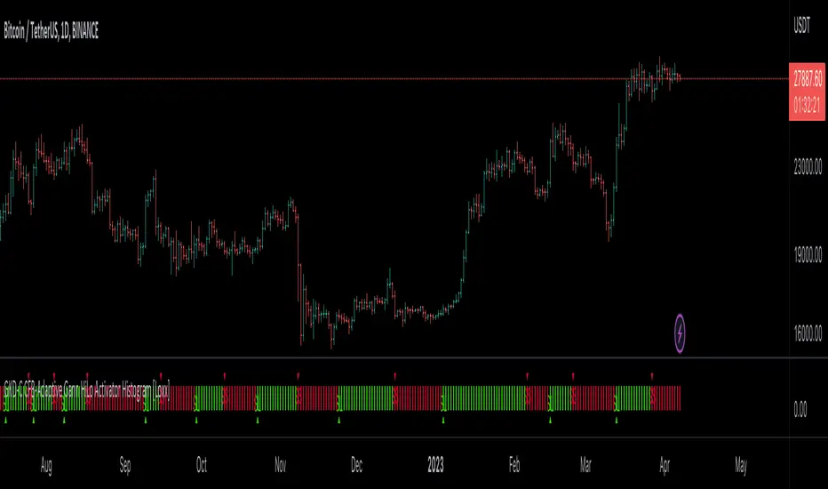
GKD-C Average Sentiment Oscillator [Loxx]The Giga Kaleidoscope GKD-C Average Sentiment Oscillator is a confirmation module included in Loxx's "Giga Kaleidoscope Modularized Trading System."
█ GKD-C Average Sentiment Oscillator
This is an older forx indicator from 2010 and represents an advancement in the formula in the sentiment meter called "FX Multimeter III." It's recommended as a precise method for assessing the sentiment over a specific candlestick duration, suitable for trend filtering or determining entry/exit points.
The oscillator merges two similar algorithms, each with a unique application:
Individual Bar Analysis: This method evaluates the bullish or bearish nature of each bar through OHLC prices, and then averages the percentages over a specified bar group (e.g., 10 bars) to derive the final sentiment percentage. While it provides a detailed intra-bar sentiment, it tends to be more volatile.
Grouped Bar Analysis: This approach views the group of bars as a singular unit, determining the sentiment based on the OHLC values of the entire group. It delivers a more consistent outcome and emphasizes broader price movement ranges.
Within the indicator settings, users can opt for these algorithms independently as Mode 1 and Mode 2, or combine them under Mode 0.
█ Giga Kaleidoscope Modularized Trading System
Core components of an NNFX algorithmic trading strategy
The NNFX algorithm is built on the principles of trend, momentum, and volatility. There are six core components in the NNFX trading algorithm:
1. Volatility - price volatility; e.g., Average True Range, True Range Double, Close-to-Close, etc.
2. Baseline - a moving average to identify price trend
3. Confirmation 1 - a technical indicator used to identify trends
4. Confirmation 2 - a technical indicator used to identify trends
5. Continuation - a technical indicator used to identify trends
6. Volatility/Volume - a technical indicator used to identify volatility/volume breakouts/breakdown
7. Exit - a technical indicator used to determine when a trend is exhausted
8. Metamorphosis - a technical indicator that produces a compound signal from the combination of other GKD indicators*
*(not part of the NNFX algorithm)
What is Volatility in the NNFX trading system?
In the NNFX (No Nonsense Forex) trading system, ATR (Average True Range) is typically used to measure the volatility of an asset. It is used as a part of the system to help determine the appropriate stop loss and take profit levels for a trade. ATR is calculated by taking the average of the true range values over a specified period.
True range is calculated as the maximum of the following values:
-Current high minus the current low
-Absolute value of the current high minus the previous close
-Absolute value of the current low minus the previous close
ATR is a dynamic indicator that changes with changes in volatility. As volatility increases, the value of ATR increases, and as volatility decreases, the value of ATR decreases. By using ATR in NNFX system, traders can adjust their stop loss and take profit levels according to the volatility of the asset being traded. This helps to ensure that the trade is given enough room to move, while also minimizing potential losses.
Other types of volatility include True Range Double (TRD), Close-to-Close, and Garman-Klass
What is a Baseline indicator?
The baseline is essentially a moving average, and is used to determine the overall direction of the market.
The baseline in the NNFX system is used to filter out trades that are not in line with the long-term trend of the market. The baseline is plotted on the chart along with other indicators, such as the Moving Average (MA), the Relative Strength Index (RSI), and the Average True Range (ATR).
Trades are only taken when the price is in the same direction as the baseline. For example, if the baseline is sloping upwards, only long trades are taken, and if the baseline is sloping downwards, only short trades are taken. This approach helps to ensure that trades are in line with the overall trend of the market, and reduces the risk of entering trades that are likely to fail.
By using a baseline in the NNFX system, traders can have a clear reference point for determining the overall trend of the market, and can make more informed trading decisions. The baseline helps to filter out noise and false signals, and ensures that trades are taken in the direction of the long-term trend.
What is a Confirmation indicator?
Confirmation indicators are technical indicators that are used to confirm the signals generated by primary indicators. Primary indicators are the core indicators used in the NNFX system, such as the Average True Range (ATR), the Moving Average (MA), and the Relative Strength Index (RSI).
The purpose of the confirmation indicators is to reduce false signals and improve the accuracy of the trading system. They are designed to confirm the signals generated by the primary indicators by providing additional information about the strength and direction of the trend.
Some examples of confirmation indicators that may be used in the NNFX system include the Bollinger Bands, the MACD (Moving Average Convergence Divergence), and the MACD Oscillator. These indicators can provide information about the volatility, momentum, and trend strength of the market, and can be used to confirm the signals generated by the primary indicators.
In the NNFX system, confirmation indicators are used in combination with primary indicators and other filters to create a trading system that is robust and reliable. By using multiple indicators to confirm trading signals, the system aims to reduce the risk of false signals and improve the overall profitability of the trades.
What is a Continuation indicator?
In the NNFX (No Nonsense Forex) trading system, a continuation indicator is a technical indicator that is used to confirm a current trend and predict that the trend is likely to continue in the same direction. A continuation indicator is typically used in conjunction with other indicators in the system, such as a baseline indicator, to provide a comprehensive trading strategy.
What is a Volatility/Volume indicator?
Volume indicators, such as the On Balance Volume (OBV), the Chaikin Money Flow (CMF), or the Volume Price Trend (VPT), are used to measure the amount of buying and selling activity in a market. They are based on the trading volume of the market, and can provide information about the strength of the trend. In the NNFX system, volume indicators are used to confirm trading signals generated by the Moving Average and the Relative Strength Index. Volatility indicators include Average Direction Index, Waddah Attar, and Volatility Ratio. In the NNFX trading system, volatility is a proxy for volume and vice versa.
By using volume indicators as confirmation tools, the NNFX trading system aims to reduce the risk of false signals and improve the overall profitability of trades. These indicators can provide additional information about the market that is not captured by the primary indicators, and can help traders to make more informed trading decisions. In addition, volume indicators can be used to identify potential changes in market trends and to confirm the strength of price movements.
What is an Exit indicator?
The exit indicator is used in conjunction with other indicators in the system, such as the Moving Average (MA), the Relative Strength Index (RSI), and the Average True Range (ATR), to provide a comprehensive trading strategy.
The exit indicator in the NNFX system can be any technical indicator that is deemed effective at identifying optimal exit points. Examples of exit indicators that are commonly used include the Parabolic SAR, the Average Directional Index (ADX), and the Chandelier Exit.
The purpose of the exit indicator is to identify when a trend is likely to reverse or when the market conditions have changed, signaling the need to exit a trade. By using an exit indicator, traders can manage their risk and prevent significant losses.
In the NNFX system, the exit indicator is used in conjunction with a stop loss and a take profit order to maximize profits and minimize losses. The stop loss order is used to limit the amount of loss that can be incurred if the trade goes against the trader, while the take profit order is used to lock in profits when the trade is moving in the trader's favor.
Overall, the use of an exit indicator in the NNFX trading system is an important component of a comprehensive trading strategy. It allows traders to manage their risk effectively and improve the profitability of their trades by exiting at the right time.
What is an Metamorphosis indicator?
The concept of a metamorphosis indicator involves the integration of two or more GKD indicators to generate a compound signal. This is achieved by evaluating the accuracy of each indicator and selecting the signal from the indicator with the highest accuracy. As an illustration, let's consider a scenario where we calculate the accuracy of 10 indicators and choose the signal from the indicator that demonstrates the highest accuracy.
The resulting output from the metamorphosis indicator can then be utilized in a GKD-BT backtest by occupying a slot that aligns with the purpose of the metamorphosis indicator. The slot can be a GKD-B, GKD-C, or GKD-E slot, depending on the specific requirements and objectives of the indicator. This allows for seamless integration and utilization of the compound signal within the GKD-BT framework.
How does Loxx's GKD (Giga Kaleidoscope Modularized Trading System) implement the NNFX algorithm outlined above?
Loxx's GKD v2.0 system has five types of modules (indicators/strategies). These modules are:
1. GKD-BT - Backtesting module (Volatility, Number 1 in the NNFX algorithm)
2. GKD-B - Baseline module (Baseline and Volatility/Volume, Numbers 1 and 2 in the NNFX algorithm)
3. GKD-C - Confirmation 1/2 and Continuation module (Confirmation 1/2 and Continuation, Numbers 3, 4, and 5 in the NNFX algorithm)
4. GKD-V - Volatility/Volume module (Confirmation 1/2, Number 6 in the NNFX algorithm)
5. GKD-E - Exit module (Exit, Number 7 in the NNFX algorithm)
6. GKD-M - Metamorphosis module (Metamorphosis, Number 8 in the NNFX algorithm, but not part of the NNFX algorithm)
(additional module types will added in future releases)
Each module interacts with every module by passing data to A backtest module wherein the various components of the GKD system are combined to create a trading signal.
That is, the Baseline indicator passes its data to Volatility/Volume. The Volatility/Volume indicator passes its values to the Confirmation 1 indicator. The Confirmation 1 indicator passes its values to the Confirmation 2 indicator. The Confirmation 2 indicator passes its values to the Continuation indicator. The Continuation indicator passes its values to the Exit indicator, and finally, the Exit indicator passes its values to the Backtest strategy.
This chaining of indicators requires that each module conform to Loxx's GKD protocol, therefore allowing for the testing of every possible combination of technical indicators that make up the six components of the NNFX algorithm.
What does the application of the GKD trading system look like?
Example trading system:
Backtest: Multi-Ticker CC Backtest
Baseline: Hull Moving Average
Volatility/Volume: Hurst Exponent
Confirmation 1: Advance Trend Pressure as shown on the chart above
Confirmation 2: uf2018
Continuation: Coppock Curve
Exit: Rex Oscillator
Metamorphosis: Baseline Optimizer
Each GKD indicator is denoted with a module identifier of either: GKD-BT, GKD-B, GKD-C, GKD-V, GKD-M, or GKD-E. This allows traders to understand to which module each indicator belongs and where each indicator fits into the GKD system.
█ Giga Kaleidoscope Modularized Trading System Signals
Standard Entry
1. GKD-C Confirmation gives signal
2. Baseline agrees
3. Price inside Goldie Locks Zone Minimum
4. Price inside Goldie Locks Zone Maximum
5. Confirmation 2 agrees
6. Volatility/Volume agrees
1-Candle Standard Entry
1a. GKD-C Confirmation gives signal
2a. Baseline agrees
3a. Price inside Goldie Locks Zone Minimum
4a. Price inside Goldie Locks Zone Maximum
Next Candle
1b. Price retraced
2b. Baseline agrees
3b. Confirmation 1 agrees
4b. Confirmation 2 agrees
5b. Volatility/Volume agrees
Baseline Entry
1. GKD-B Baseline gives signal
2. Confirmation 1 agrees
3. Price inside Goldie Locks Zone Minimum
4. Price inside Goldie Locks Zone Maximum
5. Confirmation 2 agrees
6. Volatility/Volume agrees
7. Confirmation 1 signal was less than 'Maximum Allowable PSBC Bars Back' prior
1-Candle Baseline Entry
1a. GKD-B Baseline gives signal
2a. Confirmation 1 agrees
3a. Price inside Goldie Locks Zone Minimum
4a. Price inside Goldie Locks Zone Maximum
5a. Confirmation 1 signal was less than 'Maximum Allowable PSBC Bars Back' prior
Next Candle
1b. Price retraced
2b. Baseline agrees
3b. Confirmation 1 agrees
4b. Confirmation 2 agrees
5b. Volatility/Volume agrees
Volatility/Volume Entry
1. GKD-V Volatility/Volume gives signal
2. Confirmation 1 agrees
3. Price inside Goldie Locks Zone Minimum
4. Price inside Goldie Locks Zone Maximum
5. Confirmation 2 agrees
6. Baseline agrees
7. Confirmation 1 signal was less than 7 candles prior
1-Candle Volatility/Volume Entry
1a. GKD-V Volatility/Volume gives signal
2a. Confirmation 1 agrees
3a. Price inside Goldie Locks Zone Minimum
4a. Price inside Goldie Locks Zone Maximum
5a. Confirmation 1 signal was less than 'Maximum Allowable PSVVC Bars Back' prior
Next Candle
1b. Price retraced
2b. Volatility/Volume agrees
3b. Confirmation 1 agrees
4b. Confirmation 2 agrees
5b. Baseline agrees
Confirmation 2 Entry
1. GKD-C Confirmation 2 gives signal
2. Confirmation 1 agrees
3. Price inside Goldie Locks Zone Minimum
4. Price inside Goldie Locks Zone Maximum
5. Volatility/Volume agrees
6. Baseline agrees
7. Confirmation 1 signal was less than 7 candles prior
1-Candle Confirmation 2 Entry
1a. GKD-C Confirmation 2 gives signal
2a. Confirmation 1 agrees
3a. Price inside Goldie Locks Zone Minimum
4a. Price inside Goldie Locks Zone Maximum
5a. Confirmation 1 signal was less than 'Maximum Allowable PSC2C Bars Back' prior
Next Candle
1b. Price retraced
2b. Confirmation 2 agrees
3b. Confirmation 1 agrees
4b. Volatility/Volume agrees
5b. Baseline agrees
PullBack Entry
1a. GKD-B Baseline gives signal
2a. Confirmation 1 agrees
3a. Price is beyond 1.0x Volatility of Baseline
Next Candle
1b. Price inside Goldie Locks Zone Minimum
2b. Price inside Goldie Locks Zone Maximum
3b. Confirmation 1 agrees
4b. Confirmation 2 agrees
5b. Volatility/Volume agrees
Continuation Entry
1. Standard Entry, 1-Candle Standard Entry, Baseline Entry, 1-Candle Baseline Entry, Volatility/Volume Entry, 1-Candle Volatility/Volume Entry, Confirmation 2 Entry, 1-Candle Confirmation 2 Entry, or Pullback entry triggered previously
2. Baseline hasn't crossed since entry signal trigger
4. Confirmation 1 agrees
5. Baseline agrees
6. Confirmation 2 agrees
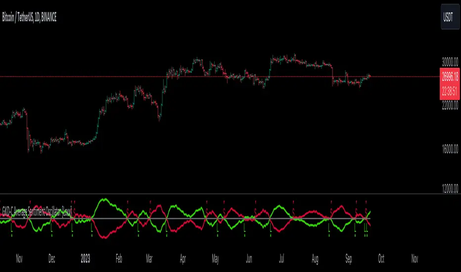
GKD-B Multi-Ticker Baseline [Loxx]Giga Kaleidoscope GKD-B Multi-Ticker Baseline is a Baseline module included in Loxx's "Giga Kaleidoscope Modularized Trading System".
This is a special implementation of GKD-B Baseline that allows the trader to input multiple tickers to be passed onto a GKD-BT Multi-Ticker Backtest. This baseline can only be used with the GKD-BT Multi-Ticker Backtests.
GKD-B Multi-Ticker Baseline includes 64 different moving averages:
Adaptive Moving Average - AMA
ADXvma - Average Directional Volatility Moving Average
Ahrens Moving Average
Alexander Moving Average - ALXMA
Deviation Scaled Moving Average - DSMA
Donchian
Double Exponential Moving Average - DEMA
Double Smoothed Exponential Moving Average - DSEMA
Double Smoothed FEMA - DSFEMA
Double Smoothed Range Weighted EMA - DSRWEMA
Double Smoothed Wilders EMA - DSWEMA
Double Weighted Moving Average - DWMA
Ehlers Optimal Tracking Filter - EOTF
Exponential Moving Average - EMA
Fast Exponential Moving Average - FEMA
Fractal Adaptive Moving Average - FRAMA
Generalized DEMA - GDEMA
Generalized Double DEMA - GDDEMA
Hull Moving Average (Type 1) - HMA1
Hull Moving Average (Type 2) - HMA2
Hull Moving Average (Type 3) - HMA3
Hull Moving Average (Type 4) - HMA4
IE /2 - Early T3 by Tim Tilson
Integral of Linear Regression Slope - ILRS
Instantaneous Trendline
Kalman Filter
Kaufman Adaptive Moving Average - KAMA
Laguerre Filter
Leader Exponential Moving Average
Linear Regression Value - LSMA ( Least Squares Moving Average )
Linear Weighted Moving Average - LWMA
McGinley Dynamic
McNicholl EMA
Non-Lag Moving Average
Ocean NMA Moving Average - ONMAMA
One More Moving Average - OMA
Parabolic Weighted Moving Average
Probability Density Function Moving Average - PDFMA
Quadratic Regression Moving Average - QRMA
Regularized EMA - REMA
Range Weighted EMA - RWEMA
Recursive Moving Trendline
Simple Decycler - SDEC
Simple Jurik Moving Average - SJMA
Simple Moving Average - SMA
Sine Weighted Moving Average
Smoothed LWMA - SLWMA
Smoothed Moving Average - SMMA
Smoother
Super Smoother
T3
Three-pole Ehlers Butterworth
Three-pole Ehlers Smoother
Triangular Moving Average - TMA
Triple Exponential Moving Average - TEMA
Two-pole Ehlers Butterworth
Two-pole Ehlers smoother
Variable Index Dynamic Average - VIDYA
Variable Moving Average - VMA
Volume Weighted EMA - VEMA
Volume Weighted Moving Average - VWMA
Zero-Lag DEMA - Zero Lag Exponential Moving Average
Zero-Lag Moving Average
Zero Lag TEMA - Zero Lag Triple Exponential Moving Average
Adaptive Moving Average - AMA
The Adaptive Moving Average (AMA) is a moving average that changes its sensitivity to price moves depending on the calculated volatility. It becomes more sensitive during periods when the price is moving smoothly in a certain direction and becomes less sensitive when the price is volatile.
ADXvma - Average Directional Volatility Moving Average
Linnsoft's ADXvma formula is a volatility-based moving average, with the volatility being determined by the value of the ADX indicator.
The ADXvma has the SMA in Chande's CMO replaced with an EMA , it then uses a few more layers of EMA smoothing before the "Volatility Index" is calculated.
A side effect is, those additional layers slow down the ADXvma when you compare it to Chande's Variable Index Dynamic Average VIDYA .
The ADXVMA provides support during uptrends and resistance during downtrends and will stay flat for longer, but will create some of the most accurate market signals when it decides to move.
Ahrens Moving Average
Richard D. Ahrens's Moving Average promises "Smoother Data" that isn't influenced by the occasional price spike. It works by using the Open and the Close in his formula so that the only time the Ahrens Moving Average will change is when the candlestick is either making new highs or new lows.
Alexander Moving Average - ALXMA
This Moving Average uses an elaborate smoothing formula and utilizes a 7 period Moving Average. It corresponds to fitting a second-order polynomial to seven consecutive observations. This moving average is rarely used in trading but is interesting as this Moving Average has been applied to diffusion indexes that tend to be very volatile.
Deviation Scaled Moving Average - DSMA
The Deviation-Scaled Moving Average is a data smoothing technique that acts like an exponential moving average with a dynamic smoothing coefficient. The smoothing coefficient is automatically updated based on the magnitude of price changes. In the Deviation-Scaled Moving Average, the standard deviation from the mean is chosen to be the measure of this magnitude. The resulting indicator provides substantial smoothing of the data even when price changes are small while quickly adapting to these changes.
Donchian
Donchian Channels are three lines generated by moving average calculations that comprise an indicator formed by upper and lower bands around a midrange or median band. The upper band marks the highest price of a security over N periods while the lower band marks the lowest price of a security over N periods.
Double Exponential Moving Average - DEMA
The Double Exponential Moving Average ( DEMA ) combines a smoothed EMA and a single EMA to provide a low-lag indicator. It's primary purpose is to reduce the amount of "lagging entry" opportunities, and like all Moving Averages, the DEMA confirms uptrends whenever price crosses on top of it and closes above it, and confirms downtrends when the price crosses under it and closes below it - but with significantly less lag.
Double Smoothed Exponential Moving Average - DSEMA
The Double Smoothed Exponential Moving Average is a lot less laggy compared to a traditional EMA . It's also considered a leading indicator compared to the EMA , and is best utilized whenever smoothness and speed of reaction to market changes are required.
Double Smoothed FEMA - DSFEMA
Same as the Double Exponential Moving Average (DEMA), but uses a faster version of EMA for its calculation.
Double Smoothed Range Weighted EMA - DSRWEMA
Range weighted exponential moving average (EMA) is, unlike the "regular" range weighted average calculated in a different way. Even though the basis - the range weighting - is the same, the way how it is calculated is completely different. By definition this type of EMA is calculated as a ratio of EMA of price*weight / EMA of weight. And the results are very different and the two should be considered as completely different types of averages. The higher than EMA to price changes responsiveness when the ranges increase remains in this EMA too and in those cases this EMA is clearly leading the "regular" EMA. This version includes double smoothing.
Double Smoothed Wilders EMA - DSWEMA
Welles Wilder was frequently using one "special" case of EMA (Exponential Moving Average) that is due to that fact (that he used it) sometimes called Wilder's EMA. This version is adding double smoothing to Wilder's EMA in order to make it "faster" (it is more responsive to market prices than the original) and is still keeping very smooth values.
Double Weighted Moving Average - DWMA
Double weighted moving average is an LWMA (Linear Weighted Moving Average). Instead of doing one cycle for calculating the LWMA, the indicator is made to cycle the loop 2 times. That produces a smoother values than the original LWMA
Ehlers Optimal Tracking Filter - EOTF
The Elher's Optimum Tracking Filter quickly adjusts rapid shifts in the price and yet is relatively smooth when the price has a sideways action. The operation of this filter is similar to Kaufman’s Adaptive Moving
Average
Exponential Moving Average - EMA
The EMA places more significance on recent data points and moves closer to price than the SMA ( Simple Moving Average ). It reacts faster to volatility due to its emphasis on recent data and is known for its ability to give greater weight to recent and more relevant data. The EMA is therefore seen as an enhancement over the SMA .
Fast Exponential Moving Average - FEMA
An Exponential Moving Average with a short look-back period.
Fractal Adaptive Moving Average - FRAMA
The Fractal Adaptive Moving Average by John Ehlers is an intelligent adaptive Moving Average which takes the importance of price changes into account and follows price closely enough to display significant moves whilst remaining flat if price ranges. The FRAMA does this by dynamically adjusting the look-back period based on the market's fractal geometry.
Generalized DEMA - GDEMA
The double exponential moving average (DEMA), was developed by Patrick Mulloy in an attempt to reduce the amount of lag time found in traditional moving averages. It was first introduced in the February 1994 issue of the magazine Technical Analysis of Stocks & Commodities in Mulloy's article "Smoothing Data with Faster Moving Averages.". Instead of using fixed multiplication factor in the final DEMA formula, the generalized version allows you to change it. By varying the "volume factor" form 0 to 1 you apply different multiplications and thus producing DEMA with different "speed" - the higher the volume factor is the "faster" the DEMA will be (but also the slope of it will be less smooth). The volume factor is limited in the calculation to 1 since any volume factor that is larger than 1 is increasing the overshooting to the extent that some volume factors usage makes the indicator unusable.
Generalized Double DEMA - GDDEMA
The double exponential moving average (DEMA), was developed by Patrick Mulloy in an attempt to reduce the amount of lag time found in traditional moving averages. It was first introduced in the February 1994 issue of the magazine Technical Analysis of Stocks & Commodities in Mulloy's article "Smoothing Data with Faster Moving Averages''. This is an extension of the Generalized DEMA using Tim Tillsons (the inventor of T3) idea, and is using GDEMA of GDEMA for calculation (which is the "middle step" of T3 calculation). Since there are no versions showing that middle step, this version covers that too. The result is smoother than Generalized DEMA, but is less smooth than T3 - one has to do some experimenting in order to find the optimal way to use it, but in any case, since it is "faster" than the T3 (Tim Tillson T3) and still smooth, it looks like a good compromise between speed and smoothness.
Hull Moving Average (Type 1) - HMA1
Alan Hull's HMA makes use of weighted moving averages to prioritize recent values and greatly reduce lag whilst maintaining the smoothness of a traditional Moving Average. For this reason, it's seen as a well-suited Moving Average for identifying entry points. This version uses SMA for smoothing.
Hull Moving Average (Type 2) - HMA2
Alan Hull's HMA makes use of weighted moving averages to prioritize recent values and greatly reduce lag whilst maintaining the smoothness of a traditional Moving Average. For this reason, it's seen as a well-suited Moving Average for identifying entry points. This version uses EMA for smoothing.
Hull Moving Average (Type 3) - HMA3
Alan Hull's HMA makes use of weighted moving averages to prioritize recent values and greatly reduce lag whilst maintaining the smoothness of a traditional Moving Average. For this reason, it's seen as a well-suited Moving Average for identifying entry points. This version uses LWMA for smoothing.
Hull Moving Average (Type 4) - HMA4
Alan Hull's HMA makes use of weighted moving averages to prioritize recent values and greatly reduce lag whilst maintaining the smoothness of a traditional Moving Average. For this reason, it's seen as a well-suited Moving Average for identifying entry points. This version uses SMMA for smoothing.
IE /2 - Early T3 by Tim Tilson and T3 new
The T3 moving average is a type of technical indicator used in financial analysis to identify trends in price movements. It is similar to the Exponential Moving Average (EMA) and the Double Exponential Moving Average (DEMA), but uses a different smoothing algorithm.
The T3 moving average is calculated using a series of exponential moving averages that are designed to filter out noise and smooth the data. The resulting smoothed data is then weighted with a non-linear function to produce a final output that is more responsive to changes in trend direction.
The T3 moving average can be customized by adjusting the length of the moving average, as well as the weighting function used to smooth the data. It is commonly used in conjunction with other technical indicators as part of a larger trading strategy.
Integral of Linear Regression Slope - ILRS
A Moving Average where the slope of a linear regression line is simply integrated as it is fitted in a moving window of length N (natural numbers in maths) across the data. The derivative of ILRS is the linear regression slope. ILRS is not the same as a SMA ( Simple Moving Average ) of length N, which is actually the midpoint of the linear regression line as it moves across the data.
Instantaneous Trendline
The Instantaneous Trendline is created by removing the dominant cycle component from the price information which makes this Moving Average suitable for medium to long-term trading.
Kalman Filter
Kalman filter is an algorithm that uses a series of measurements observed over time, containing statistical noise and other inaccuracies. This means that the filter was originally designed to work with noisy data. Also, it is able to work with incomplete data. Another advantage is that it is designed for and applied in dynamic systems; our price chart belongs to such systems. This version is true to the original design of the trade-ready Kalman Filter where velocity is the triggering mechanism.
Kalman Filter is a more accurate smoothing/prediction algorithm than the moving average because it is adaptive: it accounts for estimation errors and tries to adjust its predictions from the information it learned in the previous stage. Theoretically, Kalman Filter consists of measurement and transition components.
Kaufman Adaptive Moving Average - KAMA
Developed by Perry Kaufman, Kaufman's Adaptive Moving Average (KAMA) is a moving average designed to account for market noise or volatility. KAMA will closely follow prices when the price swings are relatively small and the noise is low.
Laguerre Filter
The Laguerre Filter is a smoothing filter which is based on Laguerre polynomials. The filter requires the current price, three prior prices, a user defined factor called Alpha to fill its calculation.
Adjusting the Alpha coefficient is used to increase or decrease its lag and its smoothness.
Leader Exponential Moving Average
The Leader EMA was created by Giorgos E. Siligardos who created a Moving Average which was able to eliminate lag altogether whilst maintaining some smoothness. It was first described during his research paper "MACD Leader" where he applied this to the MACD to improve its signals and remove its lagging issue. This filter uses his leading MACD's "modified EMA" and can be used as a zero lag filter.
Linear Regression Value - LSMA ( Least Squares Moving Average )
LSMA as a Moving Average is based on plotting the end point of the linear regression line. It compares the current value to the prior value and a determination is made of a possible trend, eg. the linear regression line is pointing up or down.
Linear Weighted Moving Average - LWMA
LWMA reacts to price quicker than the SMA and EMA . Although it's similar to the Simple Moving Average , the difference is that a weight coefficient is multiplied to the price which means the most recent price has the highest weighting, and each prior price has progressively less weight. The weights drop in a linear fashion.
McGinley Dynamic
John McGinley created this Moving Average to track prices better than traditional Moving Averages. It does this by incorporating an automatic adjustment factor into its formula, which speeds (or slows) the indicator in trending, or ranging, markets.
McNicholl EMA
Dennis McNicholl developed this Moving Average to use as his center line for his "Better Bollinger Bands" indicator and was successful because it responded better to volatility changes over the standard SMA and managed to avoid common whipsaws.
Non-lag moving average
The Non Lag Moving average follows price closely and gives very quick signals as well as early signals of price change. As a standalone Moving Average, it should not be used on its own, but as an additional confluence tool for early signals.
Ocean NMA Moving Average - ONMAMA
Created by Jim Sloman, the NMA is a moving average that automatically adjusts to volatility without being programmed to do so. For more info, read his guide "Ocean Theory, an Introduction"
One More Moving Average (OMA)
The One More Moving Average (OMA) is a technical indicator that calculates a series of Jurik-style moving averages in order to reduce noise and provide smoother price data. It uses six exponential moving averages to generate the final value, with the length of the moving averages determined by an adaptive algorithm that adjusts to the current market conditions. The algorithm calculates the average period by comparing the signal to noise ratio and using this value to determine the length of the moving averages. The resulting values are used to generate the final value of the OMA, which can be used to identify trends and potential changes in trend direction.
Parabolic Weighted Moving Average
The Parabolic Weighted Moving Average is a variation of the Linear Weighted Moving Average . The Linear Weighted Moving Average calculates the average by assigning different weights to each element in its calculation. The Parabolic Weighted Moving Average is a variation that allows weights to be changed to form a parabolic curve. It is done simply by using the Power parameter of this indicator.
Probability Density Function Moving Average - PDFMA
Probability density function based MA is a sort of weighted moving average that uses probability density function to calculate the weights. By its nature it is similar to a lot of digital filters.
Quadratic Regression Moving Average - QRMA
A quadratic regression is the process of finding the equation of the parabola that best fits a set of data. This moving average is an obscure concept that was posted to Forex forums in around 2008.
Regularized EMA - REMA
The regularized exponential moving average (REMA) by Chris Satchwell is a variation on the EMA (see Exponential Moving Average) designed to be smoother but not introduce too much extra lag.
Range Weighted EMA - RWEMA
This indicator is a variation of the range weighted EMA. The variation comes from a possible need to make that indicator a bit less "noisy" when it comes to slope changes. The method used for calculating this variation is the method described by Lee Leibfarth in his article "Trading With An Adaptive Price Zone".
Recursive Moving Trendline
Dennis Meyers's Recursive Moving Trendline uses a recursive (repeated application of a rule) polynomial fit, a technique that uses a small number of past values estimations of price and today's price to predict tomorrow's price.
Simple Decycler - SDEC
The Ehlers Simple Decycler study is a virtually zero-lag technical indicator proposed by John F. Ehlers. The original idea behind this study (and several others created by John F. Ehlers) is that market data can be considered a continuum of cycle periods with different cycle amplitudes. Thus, trending periods can be considered segments of longer cycles, or, in other words, low-frequency segments. Applying the right filter might help identify these segments.
Simple Loxx Moving Average - SLMA
A three stage moving average combining an adaptive EMA, a Kalman Filter, and a Kauffman adaptive filter.
Simple Moving Average - SMA
The SMA calculates the average of a range of prices by adding recent prices and then dividing that figure by the number of time periods in the calculation average. It is the most basic Moving Average which is seen as a reliable tool for starting off with Moving Average studies. As reliable as it may be, the basic moving average will work better when it's enhanced into an EMA .
Sine Weighted Moving Average
The Sine Weighted Moving Average assigns the most weight at the middle of the data set. It does this by weighting from the first half of a Sine Wave Cycle and the most weighting is given to the data in the middle of that data set. The Sine WMA closely resembles the TMA (Triangular Moving Average).
Smoothed LWMA - SLWMA
A smoothed version of the LWMA
Smoothed Moving Average - SMMA
The Smoothed Moving Average is similar to the Simple Moving Average ( SMA ), but aims to reduce noise rather than reduce lag. SMMA takes all prices into account and uses a long lookback period. Due to this, it's seen as an accurate yet laggy Moving Average.
Smoother
The Smoother filter is a faster-reacting smoothing technique which generates considerably less lag than the SMMA ( Smoothed Moving Average ). It gives earlier signals but can also create false signals due to its earlier reactions. This filter is sometimes wrongly mistaken for the superior Jurik Smoothing algorithm.
Super Smoother
The Super Smoother filter uses John Ehlers’s “Super Smoother” which consists of a Two pole Butterworth filter combined with a 2-bar SMA ( Simple Moving Average ) that suppresses the 22050 Hz Nyquist frequency: A characteristic of a sampler, which converts a continuous function or signal into a discrete sequence.
Three-pole Ehlers Butterworth
The 3 pole Ehlers Butterworth (as well as the Two pole Butterworth) are both superior alternatives to the EMA and SMA . They aim at producing less lag whilst maintaining accuracy. The 2 pole filter will give you a better approximation for price, whereas the 3 pole filter has superior smoothing.
Three-pole Ehlers smoother
The 3 pole Ehlers smoother works almost as close to price as the above mentioned 3 Pole Ehlers Butterworth. It acts as a strong baseline for signals but removes some noise. Side by side, it hardly differs from the Three Pole Ehlers Butterworth but when examined closely, it has better overshoot reduction compared to the 3 pole Ehlers Butterworth.
Triangular Moving Average - TMA
The TMA is similar to the EMA but uses a different weighting scheme. Exponential and weighted Moving Averages will assign weight to the most recent price data. Simple moving averages will assign the weight equally across all the price data. With a TMA (Triangular Moving Average), it is double smoother (averaged twice) so the majority of the weight is assigned to the middle portion of the data.
Triple Exponential Moving Average - TEMA
The TEMA uses multiple EMA calculations as well as subtracting lag to create a tool which can be used for scalping pullbacks. As it follows price closely, its signals are considered very noisy and should only be used in extremely fast-paced trading conditions.
Two-pole Ehlers Butterworth
The 2 pole Ehlers Butterworth (as well as the three pole Butterworth mentioned above) is another filter that cuts out the noise and follows the price closely. The 2 pole is seen as a faster, leading filter over the 3 pole and follows price a bit more closely. Analysts will utilize both a 2 pole and a 3 pole Butterworth on the same chart using the same period, but having both on chart allows its crosses to be traded.
Two-pole Ehlers smoother
A smoother version of the Two pole Ehlers Butterworth. This filter is the faster version out of the 3 pole Ehlers Butterworth. It does a decent job at cutting out market noise whilst emphasizing a closer following to price over the 3 pole Ehlers .
Variable Index Dynamic Average - VIDYA
Variable Index Dynamic Average Technical Indicator ( VIDYA ) was developed by Tushar Chande. It is an original method of calculating the Exponential Moving Average ( EMA ) with the dynamically changing period of averaging.
Variable Moving Average - VMA
The Variable Moving Average (VMA) is a study that uses an Exponential Moving Average being able to automatically adjust its smoothing factor according to the market volatility.
Volume Weighted EMA - VEMA
An EMA that uses a volume and price weighted calculation instead of the standard price input.
Volume Weighted Moving Average - VWMA
A Volume Weighted Moving Average is a moving average where more weight is given to bars with heavy volume than with light volume. Thus the value of the moving average will be closer to where most trading actually happened than it otherwise would be without being volume weighted.
Zero-Lag DEMA - Zero Lag Double Exponential Moving Average
John Ehlers's Zero Lag DEMA's aim is to eliminate the inherent lag associated with all trend following indicators which average a price over time. Because this is a Double Exponential Moving Average with Zero Lag, it has a tendency to overshoot and create a lot of false signals for swing trading. It can however be used for quick scalping or as a secondary indicator for confluence.
Zero-Lag Moving Average
The Zero Lag Moving Average is described by its creator, John Ehlers , as a Moving Average with absolutely no delay. And it's for this reason that this filter will cause a lot of abrupt signals which will not be ideal for medium to long-term traders. This filter is designed to follow price as close as possible whilst de-lagging data instead of basing it on regular data. The way this is done is by attempting to remove the cumulative effect of the Moving Average.
Zero-Lag TEMA - Zero Lag Triple Exponential Moving Average
Just like the Zero Lag DEMA , this filter will give you the fastest signals out of all the Zero Lag Moving Averages. This is useful for scalping but dangerous for medium to long-term traders, especially during market Volatility and news events. Having no lag, this filter also has no smoothing in its signals and can cause some very bizarre behavior when applied to certain indicators.
█ Volatility Goldie Locks Zone
This volatility filter is the standard first pass filter that is used for all NNFX systems despite the additional volatility/volume filter used in step 5. For this filter, price must fall into a range of maximum and minimum values calculated using multiples of volatility. Unlike the standard NNFX systems, this version of volatility filtering is separated from the core Baseline and uses it's own moving average with Loxx's Exotic Source Types.
█ Volatility Types included
The GKD system utilizes volatility-based take profits and stop losses. Each take profit and stop loss is calculated as a multiple of volatility. You can change the values of the multipliers in the settings as well.
This module includes 17 types of volatility:
Close-to-Close
Parkinson
Garman-Klass
Rogers-Satchell
Yang-Zhang
Garman-Klass-Yang-Zhang
Exponential Weighted Moving Average
Standard Deviation of Log Returns
Pseudo GARCH(2,2)
Average True Range
True Range Double
Standard Deviation
Adaptive Deviation
Median Absolute Deviation
Efficiency-Ratio Adaptive ATR
Mean Absolute Deviation
Static Percent
Various volatility estimators and indicators that investors and traders can use to measure the dispersion or volatility of a financial instrument's price. Each estimator has its strengths and weaknesses, and the choice of estimator should depend on the specific needs and circumstances of the user.
Close-to-Close
Close-to-Close volatility is a classic and widely used volatility measure, sometimes referred to as historical volatility.
Volatility is an indicator of the speed of a stock price change. A stock with high volatility is one where the price changes rapidly and with a larger amplitude. The more volatile a stock is, the riskier it is.
Close-to-close historical volatility is calculated using only a stock's closing prices. It is the simplest volatility estimator. However, in many cases, it is not precise enough. Stock prices could jump significantly during a trading session and return to the opening value at the end. That means that a considerable amount of price information is not taken into account by close-to-close volatility.
Despite its drawbacks, Close-to-Close volatility is still useful in cases where the instrument doesn't have intraday prices. For example, mutual funds calculate their net asset values daily or weekly, and thus their prices are not suitable for more sophisticated volatility estimators.
Parkinson
Parkinson volatility is a volatility measure that uses the stock’s high and low price of the day.
The main difference between regular volatility and Parkinson volatility is that the latter uses high and low prices for a day, rather than only the closing price. This is useful as close-to-close prices could show little difference while large price movements could have occurred during the day. Thus, Parkinson's volatility is considered more precise and requires less data for calculation than close-to-close volatility.
One drawback of this estimator is that it doesn't take into account price movements after the market closes. Hence, it systematically undervalues volatility. This drawback is addressed in the Garman-Klass volatility estimator.
Garman-Klass
Garman-Klass is a volatility estimator that incorporates open, low, high, and close prices of a security.
Garman-Klass volatility extends Parkinson's volatility by taking into account the opening and closing prices. As markets are most active during the opening and closing of a trading session, it makes volatility estimation more accurate.
Garman and Klass also assumed that the process of price change follows a continuous diffusion process (Geometric Brownian motion). However, this assumption has several drawbacks. The method is not robust for opening jumps in price and trend movements.
Despite its drawbacks, the Garman-Klass estimator is still more effective than the basic formula since it takes into account not only the price at the beginning and end of the time interval but also intraday price extremes.
Researchers Rogers and Satchell have proposed a more efficient method for assessing historical volatility that takes into account price trends. See Rogers-Satchell Volatility for more detail.
Rogers-Satchell
Rogers-Satchell is an estimator for measuring the volatility of securities with an average return not equal to zero.
Unlike Parkinson and Garman-Klass estimators, Rogers-Satchell incorporates a drift term (mean return not equal to zero). As a result, it provides better volatility estimation when the underlying is trending.
The main disadvantage of this method is that it does not take into account price movements between trading sessions. This leads to an underestimation of volatility since price jumps periodically occur in the market precisely at the moments between sessions.
A more comprehensive estimator that also considers the gaps between sessions was developed based on the Rogers-Satchel formula in the 2000s by Yang-Zhang. See Yang Zhang Volatility for more detail.
Yang-Zhang
Yang Zhang is a historical volatility estimator that handles both opening jumps and the drift and has a minimum estimation error.
Yang-Zhang volatility can be thought of as a combination of the overnight (close-to-open volatility) and a weighted average of the Rogers-Satchell volatility and the day’s open-to-close volatility. It is considered to be 14 times more efficient than the close-to-close estimator.
Garman-Klass-Yang-Zhang
Garman-Klass-Yang-Zhang (GKYZ) volatility estimator incorporates the returns of open, high, low, and closing prices in its calculation.
GKYZ volatility estimator takes into account overnight jumps but not the trend, i.e., it assumes that the underlying asset follows a Geometric Brownian Motion (GBM) process with zero drift. Therefore, the GKYZ volatility estimator tends to overestimate the volatility when the drift is different from zero. However, for a GBM process, this estimator is eight times more efficient than the close-to-close volatility estimator.
Exponential Weighted Moving Average
The Exponentially Weighted Moving Average (EWMA) is a quantitative or statistical measure used to model or describe a time series. The EWMA is widely used in finance, with the main applications being technical analysis and volatility modeling.
The moving average is designed such that older observations are given lower weights. The weights decrease exponentially as the data point gets older – hence the name exponentially weighted.
The only decision a user of the EWMA must make is the parameter lambda. The parameter decides how important the current observation is in the calculation of the EWMA. The higher the value of lambda, the more closely the EWMA tracks the original time series.
Standard Deviation of Log Returns
This is the simplest calculation of volatility. It's the standard deviation of ln(close/close(1)).
Pseudo GARCH(2,2)
This is calculated using a short- and long-run mean of variance multiplied by ?.
?avg(var;M) + (1 ? ?) avg(var;N) = 2?var/(M+1-(M-1)L) + 2(1-?)var/(M+1-(M-1)L)
Solving for ? can be done by minimizing the mean squared error of estimation; that is, regressing L^-1var - avg(var; N) against avg(var; M) - avg(var; N) and using the resulting beta estimate as ?.
Average True Range
The average true range (ATR) is a technical analysis indicator, introduced by market technician J. Welles Wilder Jr. in his book New Concepts in Technical Trading Systems, that measures market volatility by decomposing the entire range of an asset price for that period.
The true range indicator is taken as the greatest of the following: current high less the current low; the absolute value of the current high less the previous close; and the absolute value of the current low less the previous close. The ATR is then a moving average, generally using 14 days, of the true ranges.
True Range Double
A special case of ATR that attempts to correct for volatility skew.
Standard Deviation
Standard deviation is a statistic that measures the dispersion of a dataset relative to its mean and is calculated as the square root of the variance. The standard deviation is calculated as the square root of variance by determining each data point's deviation relative to the mean. If the data points are further from the mean, there is a higher deviation within the data set; thus, the more spread out the data, the higher the standard deviation.
Adaptive Deviation
By definition, the Standard Deviation (STD, also represented by the Greek letter sigma ? or the Latin letter s) is a measure that is used to quantify the amount of variation or dispersion of a set of data values. In technical analysis, we usually use it to measure the level of current volatility.
Standard Deviation is based on Simple Moving Average calculation for mean value. This version of standard deviation uses the properties of EMA to calculate what can be called a new type of deviation, and since it is based on EMA, we can call it EMA deviation. Additionally, Perry Kaufman's efficiency ratio is used to make it adaptive (since all EMA type calculations are nearly perfect for adapting).
The difference when compared to the standard is significant--not just because of EMA usage, but the efficiency ratio makes it a "bit more logical" in very volatile market conditions.
Median Absolute Deviation
The median absolute deviation is a measure of statistical dispersion. Moreover, the MAD is a robust statistic, being more resilient to outliers in a data set than the standard deviation. In the standard deviation, the distances from the mean are squared, so large deviations are weighted more heavily, and thus outliers can heavily influence it. In the MAD, the deviations of a small number of outliers are irrelevant.
Because the MAD is a more robust estimator of scale than the sample variance or standard deviation, it works better with distributions without a mean or variance, such as the Cauchy distribution.
For this indicator, a manual recreation of the quantile function in Pine Script is used. This is so users have a full inside view into how this is calculated.
Efficiency-Ratio Adaptive ATR
Average True Range (ATR) is a widely used indicator for many occasions in technical analysis. It is calculated as the RMA of the true range. This version adds a "twist": it uses Perry Kaufman's Efficiency Ratio to calculate adaptive true range.
Mean Absolute Deviation
The mean absolute deviation (MAD) is a measure of variability that indicates the average distance between observations and their mean. MAD uses the original units of the data, which simplifies interpretation. Larger values signify that the data points spread out further from the average. Conversely, lower values correspond to data points bunching closer to it. The mean absolute deviation is also known as the mean deviation and average absolute deviation.
This definition of the mean absolute deviation sounds similar to the standard deviation (SD). While both measure variability, they have different calculations. In recent years, some proponents of MAD have suggested that it replace the SD as the primary measure because it is a simpler concept that better fits real life.
█ Giga Kaleidoscope Modularized Trading System
Core components of an NNFX algorithmic trading strategy
The NNFX algorithm is built on the principles of trend, momentum, and volatility. There are six core components in the NNFX trading algorithm:
1. Volatility - price volatility; e.g., Average True Range, True Range Double, Close-to-Close, etc.
2. Baseline - a moving average to identify price trend
3. Confirmation 1 - a technical indicator used to identify trends
4. Confirmation 2 - a technical indicator used to identify trends
5. Continuation - a technical indicator used to identify trends
6. Volatility/Volume - a technical indicator used to identify volatility/volume breakouts/breakdown
7. Exit - a technical indicator used to determine when a trend is exhausted
8. Metamorphosis - a technical indicator that produces a compound signal from the combination of other GKD indicators*
*(not part of the NNFX algorithm)
What is Volatility in the NNFX trading system?
In the NNFX (No Nonsense Forex) trading system, ATR (Average True Range) is typically used to measure the volatility of an asset. It is used as a part of the system to help determine the appropriate stop loss and take profit levels for a trade. ATR is calculated by taking the average of the true range values over a specified period.
True range is calculated as the maximum of the following values:
-Current high minus the current low
-Absolute value of the current high minus the previous close
-Absolute value of the current low minus the previous close
ATR is a dynamic indicator that changes with changes in volatility. As volatility increases, the value of ATR increases, and as volatility decreases, the value of ATR decreases. By using ATR in NNFX system, traders can adjust their stop loss and take profit levels according to the volatility of the asset being traded. This helps to ensure that the trade is given enough room to move, while also minimizing potential losses.
Other types of volatility include True Range Double (TRD), Close-to-Close, and Garman-Klass
What is a Baseline indicator?
The baseline is essentially a moving average, and is used to determine the overall direction of the market.
The baseline in the NNFX system is used to filter out trades that are not in line with the long-term trend of the market. The baseline is plotted on the chart along with other indicators, such as the Moving Average (MA), the Relative Strength Index (RSI), and the Average True Range (ATR).
Trades are only taken when the price is in the same direction as the baseline. For example, if the baseline is sloping upwards, only long trades are taken, and if the baseline is sloping downwards, only short trades are taken. This approach helps to ensure that trades are in line with the overall trend of the market, and reduces the risk of entering trades that are likely to fail.
By using a baseline in the NNFX system, traders can have a clear reference point for determining the overall trend of the market, and can make more informed trading decisions. The baseline helps to filter out noise and false signals, and ensures that trades are taken in the direction of the long-term trend.
What is a Confirmation indicator?
Confirmation indicators are technical indicators that are used to confirm the signals generated by primary indicators. Primary indicators are the core indicators used in the NNFX system, such as the Average True Range (ATR), the Moving Average (MA), and the Relative Strength Index (RSI).
The purpose of the confirmation indicators is to reduce false signals and improve the accuracy of the trading system. They are designed to confirm the signals generated by the primary indicators by providing additional information about the strength and direction of the trend.
Some examples of confirmation indicators that may be used in the NNFX system include the Bollinger Bands, the MACD (Moving Average Convergence Divergence), and the MACD Oscillator. These indicators can provide information about the volatility, momentum, and trend strength of the market, and can be used to confirm the signals generated by the primary indicators.
In the NNFX system, confirmation indicators are used in combination with primary indicators and other filters to create a trading system that is robust and reliable. By using multiple indicators to confirm trading signals, the system aims to reduce the risk of false signals and improve the overall profitability of the trades.
What is a Continuation indicator?
In the NNFX (No Nonsense Forex) trading system, a continuation indicator is a technical indicator that is used to confirm a current trend and predict that the trend is likely to continue in the same direction. A continuation indicator is typically used in conjunction with other indicators in the system, such as a baseline indicator, to provide a comprehensive trading strategy.
What is a Volatility/Volume indicator?
Volume indicators, such as the On Balance Volume (OBV), the Chaikin Money Flow (CMF), or the Volume Price Trend (VPT), are used to measure the amount of buying and selling activity in a market. They are based on the trading volume of the market, and can provide information about the strength of the trend. In the NNFX system, volume indicators are used to confirm trading signals generated by the Moving Average and the Relative Strength Index. Volatility indicators include Average Direction Index, Waddah Attar, and Volatility Ratio. In the NNFX trading system, volatility is a proxy for volume and vice versa.
By using volume indicators as confirmation tools, the NNFX trading system aims to reduce the risk of false signals and improve the overall profitability of trades. These indicators can provide additional information about the market that is not captured by the primary indicators, and can help traders to make more informed trading decisions. In addition, volume indicators can be used to identify potential changes in market trends and to confirm the strength of price movements.
What is an Exit indicator?
The exit indicator is used in conjunction with other indicators in the system, such as the Moving Average (MA), the Relative Strength Index (RSI), and the Average True Range (ATR), to provide a comprehensive trading strategy.
The exit indicator in the NNFX system can be any technical indicator that is deemed effective at identifying optimal exit points. Examples of exit indicators that are commonly used include the Parabolic SAR, the Average Directional Index (ADX), and the Chandelier Exit.
The purpose of the exit indicator is to identify when a trend is likely to reverse or when the market conditions have changed, signaling the need to exit a trade. By using an exit indicator, traders can manage their risk and prevent significant losses.
In the NNFX system, the exit indicator is used in conjunction with a stop loss and a take profit order to maximize profits and minimize losses. The stop loss order is used to limit the amount of loss that can be incurred if the trade goes against the trader, while the take profit order is used to lock in profits when the trade is moving in the trader's favor.
Overall, the use of an exit indicator in the NNFX trading system is an important component of a comprehensive trading strategy. It allows traders to manage their risk effectively and improve the profitability of their trades by exiting at the right time.
What is an Metamorphosis indicator?
The concept of a metamorphosis indicator involves the integration of two or more GKD indicators to generate a compound signal. This is achieved by evaluating the accuracy of each indicator and selecting the signal from the indicator with the highest accuracy. As an illustration, let's consider a scenario where we calculate the accuracy of 10 indicators and choose the signal from the indicator that demonstrates the highest accuracy.
The resulting output from the metamorphosis indicator can then be utilized in a GKD-BT backtest by occupying a slot that aligns with the purpose of the metamorphosis indicator. The slot can be a GKD-B, GKD-C, or GKD-E slot, depending on the specific requirements and objectives of the indicator. This allows for seamless integration and utilization of the compound signal within the GKD-BT framework.
How does Loxx's GKD (Giga Kaleidoscope Modularized Trading System) implement the NNFX algorithm outlined above?
Loxx's GKD v2.0 system has five types of modules (indicators/strategies). These modules are:
1. GKD-BT - Backtesting module (Volatility, Number 1 in the NNFX algorithm)
2. GKD-B - Baseline module (Baseline and Volatility/Volume, Numbers 1 and 2 in the NNFX algorithm)
3. GKD-C - Confirmation 1/2 and Continuation module (Confirmation 1/2 and Continuation, Numbers 3, 4, and 5 in the NNFX algorithm)
4. GKD-V - Volatility/Volume module (Confirmation 1/2, Number 6 in the NNFX algorithm)
5. GKD-E - Exit module (Exit, Number 7 in the NNFX algorithm)
6. GKD-M - Metamorphosis module (Metamorphosis, Number 8 in the NNFX algorithm, but not part of the NNFX algorithm)
(additional module types will added in future releases)
Each module interacts with every module by passing data to A backtest module wherein the various components of the GKD system are combined to create a trading signal.
That is, the Baseline indicator passes its data to Volatility/Volume. The Volatility/Volume indicator passes its values to the Confirmation 1 indicator. The Confirmation 1 indicator passes its values to the Confirmation 2 indicator. The Confirmation 2 indicator passes its values to the Continuation indicator. The Continuation indicator passes its values to the Exit indicator, and finally, the Exit indicator passes its values to the Backtest strategy.
This chaining of indicators requires that each module conform to Loxx's GKD protocol, therefore allowing for the testing of every possible combination of technical indicators that make up the six components of the NNFX algorithm.
What does the application of the GKD trading system look like?
Example trading system:
Backtest: Multi-Ticker SCC Backtest
Baseline: Hull Moving Average
Volatility/Volume: Hurst Exponent
Confirmation 1: Fisher Trasnform
Confirmation 2: uf2018
Continuation: Vortex
Exit: Rex Oscillator
Metamorphosis: Baseline Optimizer
Each GKD indicator is denoted with a module identifier of either: GKD-BT, GKD-B, GKD-C, GKD-V, GKD-M, or GKD-E. This allows traders to understand to which module each indicator belongs and where each indicator fits into the GKD system.
█ Giga Kaleidoscope Modularized Trading System Signals
Standard Entry
1. GKD-C Confirmation gives signal
2. Baseline agrees
3. Price inside Goldie Locks Zone Minimum
4. Price inside Goldie Locks Zone Maximum
5. Confirmation 2 agrees
6. Volatility/Volume agrees
1-Candle Standard Entry
1a. GKD-C Confirmation gives signal
2a. Baseline agrees
3a. Price inside Goldie Locks Zone Minimum
4a. Price inside Goldie Locks Zone Maximum
Next Candle
1b. Price retraced
2b. Baseline agrees
3b. Confirmation 1 agrees
4b. Confirmation 2 agrees
5b. Volatility/Volume agrees
Baseline Entry
1. GKD-B Basline gives signal
2. Confirmation 1 agrees
3. Price inside Goldie Locks Zone Minimum
4. Price inside Goldie Locks Zone Maximum
5. Confirmation 2 agrees
6. Volatility/Volume agrees
7. Confirmation 1 signal was less than 'Maximum Allowable PSBC Bars Back' prior
1-Candle Baseline Entry
1a. GKD-B Baseline gives signal
2a. Confirmation 1 agrees
3a. Price inside Goldie Locks Zone Minimum
4a. Price inside Goldie Locks Zone Maximum
5a. Confirmation 1 signal was less than 'Maximum Allowable PSBC Bars Back' prior
Next Candle
1b. Price retraced
2b. Baseline agrees
3b. Confirmation 1 agrees
4b. Confirmation 2 agrees
5b. Volatility/Volume agrees
Volatility/Volume Entry
1. GKD-V Volatility/Volume gives signal
2. Confirmation 1 agrees
3. Price inside Goldie Locks Zone Minimum
4. Price inside Goldie Locks Zone Maximum
5. Confirmation 2 agrees
6. Baseline agrees
7. Confirmation 1 signal was less than 7 candles prior
1-Candle Volatility/Volume Entry
1a. GKD-V Volatility/Volume gives signal
2a. Confirmation 1 agrees
3a. Price inside Goldie Locks Zone Minimum
4a. Price inside Goldie Locks Zone Maximum
5a. Confirmation 1 signal was less than 'Maximum Allowable PSVVC Bars Back' prior
Next Candle
1b. Price retraced
2b. Volatility/Volume agrees
3b. Confirmation 1 agrees
4b. Confirmation 2 agrees
5b. Baseline agrees
Confirmation 2 Entry
1. GKD-C Confirmation 2 gives signal
2. Confirmation 1 agrees
3. Price inside Goldie Locks Zone Minimum
4. Price inside Goldie Locks Zone Maximum
5. Volatility/Volume agrees
6. Baseline agrees
7. Confirmation 1 signal was less than 7 candles prior
1-Candle Confirmation 2 Entry
1a. GKD-C Confirmation 2 gives signal
2a. Confirmation 1 agrees
3a. Price inside Goldie Locks Zone Minimum
4a. Price inside Goldie Locks Zone Maximum
5a. Confirmation 1 signal was less than 'Maximum Allowable PSC2C Bars Back' prior
Next Candle
1b. Price retraced
2b. Confirmation 2 agrees
3b. Confirmation 1 agrees
4b. Volatility/Volume agrees
5b. Baseline agrees
PullBack Entry
1a. GKD-B Baseline gives signal
2a. Confirmation 1 agrees
3a. Price is beyond 1.0x Volatility of Baseline
Next Candle
1b. Price inside Goldie Locks Zone Minimum
2b. Price inside Goldie Locks Zone Maximum
3b. Confirmation 1 agrees
4b. Confirmation 2 agrees
5b. Volatility/Volume agrees
Continuation Entry
1. Standard Entry, 1-Candle Standard Entry, Baseline Entry, 1-Candle Baseline Entry, Volatility/Volume Entry, 1-Candle Volatility/Volume Entry, Confirmation 2 Entry, 1-Candle Confirmation 2 Entry, or Pullback entry triggered previously
2. Baseline hasn't crossed since entry signal trigger
4. Confirmation 1 agrees
5. Baseline agrees
6. Confirmation 2 agrees
█ Connecting to Backtests
All GKD indicators are chained indicators meaning you export the value of the indicators to specialized backtest to creat your GKD trading system. Each indicator contains a proprietary signal generation algo that will only work with GKD backtests. You can find these backtests using the links below.
GKD-BT Giga Confirmation Stack Backtest
GKD-BT Giga Stacks Backtest
GKD-BT Full Giga Kaleidoscope Backtest
GKD-BT Solo Confirmation Super Complex Backtest
GKD-BT Solo Confirmation Complex Backtest
GKD-BT Solo Confirmation Simple Backtest
GKD-M Baseline Optimizer
GKD-M Accuracy Alchemist

[delta2win] ShockSentinel Early Warnings🚀 ShockSentinel Early Warnings — Advanced Multi-Symbol Shock Detection System
📊 UNIQUE METHODOLOGY:
This indicator implements a proprietary concordance-based shock detection system that goes beyond simple price movement analysis. Unlike basic pump/dump detectors, it uses a sophisticated multi-symbol correlation algorithm to validate signals across multiple assets simultaneously, significantly reducing false positives while maintaining sensitivity to genuine market shocks.
🔬 TECHNICAL APPROACH:
• Adaptive Threshold System: Automatically adjusts detection sensitivity based on timeframe using proprietary scaling algorithms:
- 1m: 0.5% threshold (ultra-sensitive for scalping)
- 3m: 1.0% threshold (high-frequency trading)
- 5m: 2.0% threshold (short-term momentum)
- 15m: 3.0% threshold (intraday swings)
- 1h: 6.0% threshold (daily moves)
- 4h+: 10.0% threshold (swing trading)
• Dual Detection Modes:
- Percent Mode: Calculates maximum percentage change within configurable lookback window (1-6 bars) using the formula: max(|(close - close ) / close * 100|) for i = 1 to window
- ATR-Normalized Mode: Uses Average True Range for volatility-adjusted detection across different market regimes: max(|close - close | / ATR) for i = 1 to window
• Concordance Algorithm: Proprietary multi-symbol validation system that requires minimum correlation count across up to 4 additional symbols, ensuring signals are validated by market-wide participation rather than isolated price movements
• Non-Repainting Architecture: Optional bar-close confirmation prevents false signals from intraday noise while maintaining real-time alert capability for immediate response
🎯 MATHEMATICAL FOUNDATION:
The core algorithm implements a sliding window maximum change detection:
Percent Change Calculation:
For each bar, the system calculates the maximum absolute percentage change over the specified window:
- PctChange = (close - close ) / close * 100
- MaxPct = max(|PctChange |) for i = 1 to window
- Signal triggers when MaxPct >= threshold
ATR-Normalized Calculation:
For volatility-adjusted detection:
- ATRChange = (close - close ) / ATR
- MaxATR = max(|ATRChange |) for i = 1 to window
- Signal triggers when MaxATR >= ATR_multiplier
Concordance Validation:
- Requires minimum N symbols showing same directional movement
- Validates signal strength through market participation
- Reduces false signals from isolated price movements
- Improves signal quality through correlation analysis
⚙️ ADVANCED FEATURES:
• Preset System: 7 pre-configured strategies with optimized parameters:
- Scalp (Ultra-Fast): 0.6x scaling, 2-bar window, real-time alerts
- Aggressive: 0.7x scaling, 2-bar window, real-time alerts
- Balanced: 1.0x scaling, 3-bar window, confirmed signals
- Conservative: 1.3x scaling, 4-bar window, confirmed signals
- Volatility-Adaptive: ATR mode, 7-period ATR, 2.5x multiplier
- Momentum (Intraday): ATR mode, 10-period ATR, 2.0x multiplier
- Swing (Slow): ATR mode, 14-period ATR, 2.8x multiplier
• Real-time vs Confirmed: Choose between immediate alerts or bar-close confirmation
• Visual Analytics: Integrated signal history table with concordance gauges and performance metrics
• Professional Alerts: Multi-format alert system (Compact, Extended, Plain, CSV) with Telegram integration and customizable messaging
💡 UNIQUE VALUE PROPOSITION:
Unlike simple price change detectors, this system provides:
1. Multi-Symbol Validation: Validates signals across multiple correlated assets, ensuring market-wide participation
2. Adaptive Thresholds: Automatically adjusts sensitivity based on timeframe and market conditions
3. Dual Signal Types: Provides both real-time and confirmed signal options for different trading styles
4. Comprehensive Analytics: Includes signal history, concordance gauges, and performance tracking
5. Advanced Concordance: Uses sophisticated correlation algorithms for signal validation
6. Professional Integration: Built-in Telegram support with customizable message formats
🔧 USAGE INSTRUCTIONS:
1. Select Preset: Choose appropriate strategy for your trading style and timeframe
2. Configure Symbols: Add up to 4 additional symbols for concordance validation
3. Set Concordance: Adjust minimum count (higher = more selective, lower = more sensitive)
4. Choose Mode: Select between real-time or confirmed signals based on your risk tolerance
5. Enable Alerts: Configure notification preferences and message formats
6. Monitor Performance: Use integrated tables to track signal quality and concordance
📈 PERFORMANCE CHARACTERISTICS:
• Optimized for Crypto: Designed specifically for high-volatility cryptocurrency markets
• Multi-Timeframe: Effective across all timeframes from 1-minute to 4-hour charts
• False Signal Reduction: Multi-symbol validation significantly reduces false positives
• Flexible Sensitivity: Adjustable thresholds allow customization for different market conditions
• Real-time Capability: Provides immediate alerts for fast-moving markets
• Confirmation Option: Bar-close confirmation for conservative trading approaches
⚠️ TECHNICAL CONSIDERATIONS:
• Real-time Mode: May generate multiple alerts per bar; use cooldown settings to manage frequency
• Data Dependencies: Concordance requires data availability for all configured symbols
• Market Regimes: ATR mode provides better performance in varying volatility conditions
• Signal Quality: Higher concordance requirements reduce false signals but may miss opportunities
• Latency: request.security calls depend on data provider latency and availability
🎯 TARGET MARKETS:
• Cryptocurrency Trading: High-volatility crypto markets with frequent shock events
• Scalping: Short-term trading strategies requiring immediate signal detection
• Swing Trading: Medium-term strategies benefiting from confirmed signals
• Portfolio Management: Multi-asset correlation analysis for risk management
• Algorithmic Trading: Systematic strategies requiring reliable signal validation
📊 SIGNAL INTERPRETATION:
• Green Arrows (Pump): Upward price shock with sufficient concordance
• Red Arrows (Dump): Downward price shock with sufficient concordance
• Large Markers: Confirmed signals with high concordance
• Small Markers: Early signals with lower concordance
• Background Colors: Visual intensity based on concordance strength
• Tables: Historical signal tracking with performance metrics
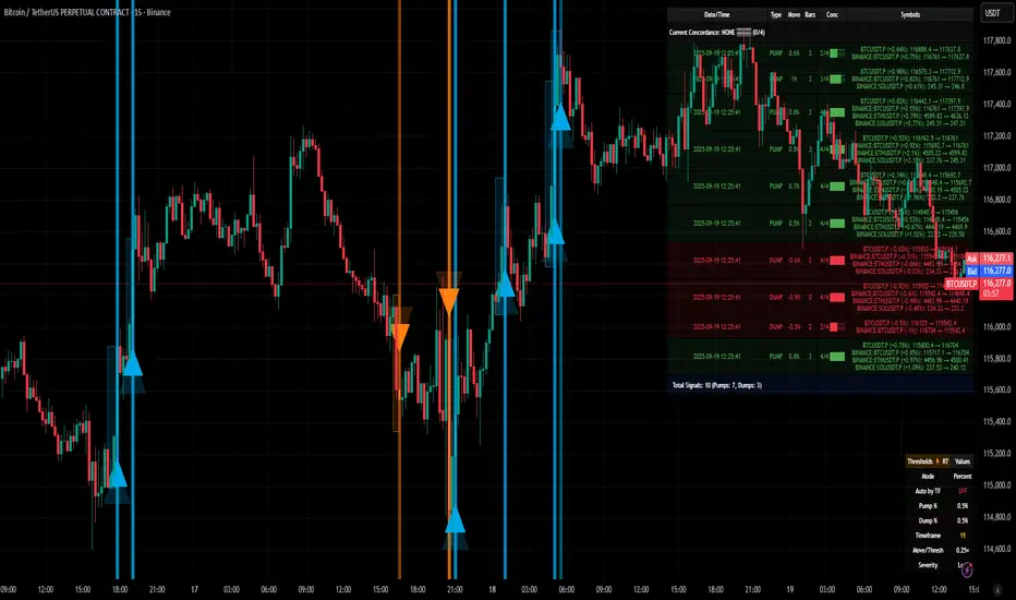
[Excalibur][Pandora][Mosaic] Ultra Spectrum Analyzer@veryfid, you will always be remembered eternally...
ANCIENT MYTHOS AND LORE:
The retellings of "Pandora's Box" serve as a cautionary metaphor depicting an opened container (pithos - jar) that once held profound perils and evils — sufferings that are experienced around the world in various forms. The known and vague mythical box contents actually represent manifestation of evils, situational adversities, and human disparities that have been encountered throughout life for aeons. In contemporary times, a meager list of ordeals would include incidents of deceit, betrayal, corruption, oppression, greed, envy, depravity, conflict, mania, affliction, plague, and mortality. However, as the tale is told, kept and remaining inside the box was the essence of expectant hope (elpis), which may represent the optimism and resilience to overcome immense hardships.
There are other versions of the classic story where Pandora isn't actually the culprit, being her husband Epimetheus was the lid lifting perpetrator and the one who always and actually received the gift(s). Curiously, the interpreted Greek word ‘Pandora’ translated to English, can mean either "all-endowed" or "all-gifting". Much like Pandora herself, who was formed from clay of the earth, the jar also would have been most likely crafted from clay. Conceived as a made-to-order maiden for an arranged marriage, Pandora was given qualities of exquisite beauty, persuasive charm, all while being adorned with jewelry and fine clothing. Olympian premeditated preparations in the didactic fable of 'Works and Days' by Hesiod had blamable intent and would be later used for centuries as denigration of women/mothers. The rest of Hesiod's tale is even worse.
In reality, the entire contrived exploit of incarnating Pandora as a trojan temptress was solely intended as an instrument of infiltration and entrapment for delivery to Epimetheus as an arranged seductive snare. Being a man myself, I find it appalling how the antiquated writings of ancient morphological men have repeatedly ostracized women for many of the ailments of mankind. When in truth, it is far more often that despicable men are the recorded all time winning historical harbingers of global abysmal darkness by means of ideological treachery. Vast historical chronicles since antiquity have frequently recorded who the typical real-world villains truly are and are not. As the stories are told in the first place, it was dictator Zeus along with his Olympian conspirators, who intently implanted malicious spirits into a gifted receptacle to orchestrate planetary suffering and carnage on humankind.
PROLOGUE:
I believe, it is way past overdue to restore Pandora's name to a place of better standing. As I have been peaking into a theoretical pitcher of mathematic mysteria for years now, where no one else dares to look. Once upon a time, I pondered an opposite notion: What if Pandora was originally conceived to solve global problems instead of creating them? Maybe Pandora could have been wielded into existence to wage unrelenting and avenging retribution on every dominance hierarchy and each diabolical enemy intently hostile to humankind. My hypothetical version of Pandora would take the notion of "mors omnibus tyrannis" to a whole other fearsome magnitude. She would cause evil arrogant men to tremble with sheer horror... the kind of fear ALL false gods, despotic kings, tyrannical dictators, controligarchies, and criminal syndicates truly worry about at night. In my opinion, that would be a better fictional story worthy of retelling for aeons.
One unique goliath 21st century adversary is LAG and it must be subdued or minimized. This unyielding nemesis is also known as group delay, processing delay, and algorithmic latency. My eyes are locked onto this opponent with fixation that will never surrender a staring contest. The formidable creature lag is my daily arch enemy destined for defeat in battle. It's losing time after time and bar by bar during the past year of 2023. In my attempts to peer through the murky darkness of useless and deceptive information, I am confident that I have found more suitable answers to many current dilemmas of algorithmic lag.
The internet, using mathematics and the speed of light as a planetary beneficial advantage, has already performed wonders by drastically reducing the delay of dissemination of knowledge. This has garnered a mostly positive rapid acceleration of economic evolution. However, hierarchies of dark forces of chaos and subversion by the thousands lurking in the global shadows are not thrilled about well informed populations. In the present era, new spectrums of strife within planetary societies are being waged, one of the worst forms taking the hideous form of censorship. Other nefarious tactics are hindering economic progress with substantial negativity using heavily funded penetration and infiltration operations. Those sinister operational varieties are spanning psychological, cultural, educational, digital, financial, electoral, scientific, medical, biological, commercial, infrastructural, institutional, and organizational domains.
They are mistakenly meddling with the entire primordial order of planetary natural dynamics. The miscalculations from these malevolent CAUSES will be countered with EFFECTS of immense retaliatory primal veracity having equal or exceedingly more powerful opposition with overwhelming numbers in mass. It is a law embedded within the universe that supersedes ALL laws, known as 'causality'. Everyone, especially programmers, know exactly what to do with predatory infiltrating cockroaches... When tyranny becomes enforced law by agendized policies in any land, order = abs(DUTY) * pow(RIGHT) * exp(PEOPLE).
FUTURE ECONOMIC ADVERSARIAL CHALLENGES:
Just as programmers have to critically analyze our code for BUGS, a scrutinized analysis of the current world around us is at times necessary. It is an empirical statistical fact that a few percent of captains at the helm of industry, commerce, institutes, and governance are monetarily psychopathic. They are often hidden bugs operating within national systems. The subsequent economic consequences result in effects that aren't always clearly obvious to all. Here are a few global economic security issues...
Corrupted immoral code in national operation is an inevitable breakdown waiting to happen. In the harsh future to follow, old degenerate interdependent control systems will need to be dismantled and discarded, eventually succeeded by having resilient parallel arrangements with robust independent fidelity. The coming successive paradigm shifts would include future hardware and the hefty novel algorithms that will run on them afterwards. Evolution is inevitable! The internet must be upgraded and continually programmed securely to the near hardness of diamonds at multiple layers within the operational code to retain peaceful global integrity between international collaborations.
DigitalID is never going to fix an insecure vulnerable titanic network of devices full of holes taking in megatons of water from every direction. Weaponized digital mucking ID dead on arrival is certainly NOT a one size fits all solution and it still doesn't do diddly-squat to secure the internet's DNA as executable code. DigID's real purpose is to manage servitude digitally and keep citizens right where they want them, as subservient slaves.
There is a very specific reason why we have key chain rings in OUR pockets with numerous private keys evolving technologically over time to robustly safeguard individual locks we use every day, duh. AI becoming an artificial sentient hyper intelligence may sooner or later become a potential hazard, especially if it breaks AES192 into a thousand shards of glass. Perilous aspects from artilects will emerge and are coming swiftly. AI is already being weaponized and tasked to mind muzzle expressions of human consciousness.
Also, EMPs from the sun ARE an imminent planetary threat, and no amount of carbon taxation schemes inciting anthropomorphic climate hysteria originating from falsified modeling hocus-pocus is going to protect against extreme solar cycle related X-class phenomena. Our solar system candle called the sun, is not consistently energy irradiation stable if you just glance at SOHO images/video. There are very obvious cyclical frequencies within the dynamics of the sun's energetic activity that affect planets far beyond earth. The earth already has a built-in natural thermometer indicating that oceans have been rising very linearly for thousands of years since the last ice age, submerging entire ancient cities under coastal water dozens of meters.
BEAR with me and pardon my French translation, but I have the option to call major league climate BULLshite. There is no hardcore "anthropomorphic climate crisis" proof. It is a crisis in failed modeling that is insufficient to properly estimate colossal computations with dircet limited empirical data with enough accuracy to anticipate higly probable future outcomes. People deserve solid science instead of slanderous smackdowns and slighted statistics. 400ppm of atmospheric CO2 is nothing compared to previously existing 1600ppm concentrations acquired from ancient indirect historical observations at a time when early humans were hunter gatherers driving gas guzzlers.
Western climate-monger fortune tellers are scamming every nation on earth, betraying the collective human species worldwide by climate hype strangulation. Wait until the sheeple with dinner forks turn on the rabid wolves in shepherds's clothing; it has already begun. What these predatory profiteering fraudsters are not telling you is WATER (H2O) in earth's atmosphere is the all time dominating and potent greenhouse gas, always has been, not CO2. Dr. Willie Soon has explained it in the best of ways with clarity. Misleaders, banksterCorpses, and mediaPresstitutes are immensely involved in this hot model scheme and like keeping people right where they want them, force fed with mental filth with regularly scheduled socially engineered programming.
Beware of agendas and isms. The ESGovernanceAgenda is ready made economic coffin nails. I'll explain this very simply, a future green war on carbon is a silent war on carbon lifeforms and economies. Many of the smiling faces you can actually see on the world stage pulling levers are often the coldest blooded deceivers beyond anything you can ever imagine. In truth, corporate agents and policies are the greatest devastators to ecologies, while in concert, they are incessantly waging blame campaign agendas with subversive narratives by targeting consumers as the wrongdoers.
Why am I mentioning all these adversarial difficulties? Well, the intertangling myriads of tomorrow's "bundle of burdens" in a future box ALL have to be thoroughly analyzed, sifted through, and dealt with tenaciously now and in the future by generations to come in every nation state. Some days I wonder if Hesiod's fiction was taken from reality over 2000 years ago to WARN future world inhabitants. In the scope of economics, the series of incidents that have or will lead up to major world events, will need to have the frequency of related occurrences examined that lead up to crucial points in time historically. In order to prevent future disparities, our progeny will look backwards into history with ultra clarity and vigilance to see how corrupted society once was by hordes of overlords twisted by obsessive delusions of absolute power over the entire human species. There is no human race, only diverse genetic multiformity expressed from the DNA code of humankind exists.
We can't simply put the lid back on low entropy hydroCarbons and a broadband globalNet without having an implemented proven replacement or upgrade. It's far too late, leaving only wiser security chess moves forward as the only viable options. Nikola Tesla was dreaming of this daily in order to build every foundation of modern civilization that we now enjoy today and take for granted. Humanity still has to evolve by unlocking hidden secrets of mother nature. For instance, nations powered by endless geothermal electricity and deuterium fusion WILL solve a lot of the world's problems. Imagine our world dominantly powered by extreme abundant amounts of heavy water... Lady destiny awaits and begs for the future to be built securely, by eventual abandonment of antiquated wheelworks that eventually deserve to be hurled into the annihilatory dustbin of history.
SPECTRAL BURDENS:
Ephemeral 'spectral contents' are extremely difficult to decipher with the least amount of lag, especially while they reside within a noise ridden non-stationary environment. When 'lifting the lid off' of series analysis to peek with quick discernment, distinguishing between real-time relevant signals differing from intertwining undesirable randomness in a crowded information space, requires special kinds of intricate extraction. Due to the nature of fractal chaos, any novel spectral method is better than the scanty few we have now. Firstly, let's comprehend agilities of interpreting a spectrum's structure...
SPECTRAL ANALYSIS PURPOSE AND INTENTION:
Frequency Analysis - Spectral analysis serves a crucial purpose in unraveling the frequency composition of a signal. Its primary intention is to explore the intricacies of a dataset by identifying dominant frequencies and unveiling inherent cyclical patterns. This foundational understanding forms the basis for improving analyses.
Power Spectrum Visualization - The visualization of a signal's power spectrum is a key objective in spectral analysis. By portraying how power is distributed across different frequencies, the goal is to provide a visual representation of the signal's energy landscape. This insight aids with grasping the significance of various frequency components obtained from a larger whole.
Signal Characteristics - Understanding the traits of a signal is another vital goal. Spectral analysis seeks to characterize the nature of the signal, unveiling its periodicity, trends, or irregularities. This knowledge is instrumental in deciphering the behavior of the signal over time, fostering a deeper comprehension.
Algorithmic Adaptation - Spectral analyzer estimation can play a pivotal role in algorithmic development. By assisting with the creation of algorithms sensitive to specific frequency ranges, one possible advantage is to enable real-time adaptability. This adaptability approach may allow algorithms to respond dynamically to variations in different spectral components, potentially enhancing their efficacy.
Market Analysis - In the realm of trading systems and financial markets, spectral analysis methods can serve as applicable functions when studying market dynamics. By 'uncovering' trends, cycles, and anomalies within financial instruments, this analytical proficiency can aid traders and algorithm developers with making better informed decisions based on the spectral attributes of market data.
Noise/Interference Detection - Another purpose of spectral analysis is to identify and scrutinize undesirable elements within a signal, such as noise or interference. One benefit would be to facilitate the development of strategies to mitigate or eliminate these unwanted components, ultimately refining the quality of a given signal with filtration.
INTRODUCTION:
Allow me to introduce Pandora! What you see in the demonstration above, I've named it "Pandora Periodogram", which is also referred to as 'Ultra Spectrum Analyzer' (USA) for technical minds. Firstly, this is NOT technically speaking an indicator like most others. I would describe it as an avant-garde cycle period detector obtaining accurate spectral estimates on market data with Pine Script v5.0. USA is a spectral analysis cryptid that I can only describe as being an alien saber in nature. It is my rendering of spectral wrath unleashed. With time and history to come, my HOPE is this instrument will reveal Excalibur like aspects capable of slicing up a spectrum craftily, traits long thought to be a mythical enigma.
It is not modified forms of either Autocorrelation Periodogram (ACP) or MESA. Pandora's Periodogram embodies an entirely distinct design, adorned with glamourous color, by incorporating several of my most profound, highly refined technological innovations that I have poetically composed into being. What I have forged in Pine, has essentially manifested as a zero lag spectrum analyzer. Pandora easily peeks inside a single signal source more effectively to inspect for hidden spectres, revealing invisible apparitions inside data with improved clarity...
My 'Ultra Spectrum Analyzer' bears an eerie likeness to Autocorrelation Periodogram, but it possesses no autocorrelation and the other small hindrances of ACP that I formerly encountered. While ACP does have a few shortcomings, a few bars of lag, and high frequency bias, it is still phenomenal code. ACP is one answer to spectral enigmas, but not the only one. Developers can utilize this detector by creating scripts that employ a "Dominant Cycle Source" input to adaptively govern algorithms. If you are capable of building suitable algorithms for direct tethering to Autocorrelation Periodogram, then this is your next step in evolutionary application to tether to when you are ready. ACP is a good place to start building upon as an exploratory vessel, before you might ponder using USA. Once you do obtain dynamic ACP sweetness with only a few pesky bars of dominant cycle induced lag, USA may be your tool chest choice without the burden of subtle ACP lag.
USA is possibly the end of my quest for spectral bliss, for the time being. However, I still suspect there is more room for upgrades to Pandora in the future. I must mention, as an overture, this won't be the last of Pandora tech that you will witness, as my literal "out of the box thinking" will unleash many additional creations upon this Earth. The "Power of Pine" merely serves as the beginning foundational phase... Some of my futuristic dreams and daydreams of TradingView are droplets in a wavy ocean of economic providence and potential.
What I am crafting in poetic form is born out of raw curiosity. Future creations are probably best kept private for now, but I will present my future tech with beauty and elegance as it should rightfully be. There's one catch, I have absolutely no idea what this and my future marvels may do to the future of digital signal processing (DSP) and markets. I do fear any insane AI or MALEficent entity ever seeing this code. My innermost hopes and ambitions are always focused on achieving the best result obtainable. What the future can hold, may be absolutely exquisite to gaze upon, maybe even monstrous, or possibly a combination of both.
Notice: Unfortunately, I will not provide any integration support into member's projects at all. My own projects demand too much of my day to day time. I hope you understand. Meanwhile, I'll be applying this on future indication until Mr. Mortality sneaks up behind me.
FEATURES AND CHARACTERISTICS:
I have included as much ultra adjustability as I can humanly muster. Those features being the following and more...
Color Preferences - Four vivid color schemes are available in the original release. The "Ultra Violet" color scheme, in particular, contributes to the indicator's technical title, as it seems to me to reveal the greatest detail of my various spectral color schemes. Color inversion of the four color schemes is also possible, yielding eight schemes in total with predator style visuals. Heatmap transparency control is also provided.
Lag Control - Pandora achieves zero lag spectral approximations, with the added capability to control lag using an input for selectable delay. Note, however, that testing less than zero lag has not been assessed thoroughly due to potential unforeseen instability concerns. Adjustments are provided in either direction for further testing.
Spectral Bias Mitigation - Options for mitigating high OR low-frequency spectral biases are present. One interesting tweak made during development was a subtle form of spectral manipulation, involving a partial reduction of frequency amplitudes influencing either the highest or lowest periodicities. This slightly reduces the impact on the upper and lower portions of the spectrogram and the dominant cycle measurement. What initially surfaced as an unexpected discovery, may now be considered worthy of experimental utility.
Adjustable Periodogram Window Size - The periodogram is adjustable for various window sizes of periodic operation. Exploration up to a periodicity of 59 is obtainable for curiosity's sake. This flexibility challenges the notion that curiosity isn't always a negative trait, contrasting with Hesiod's ancient perspective.
Dominant Cycle Filtration - Filtration of the dominant cycle is achieved with a novel smoother having reduced lag, easily surpassing SuperSmoother's performance. However, defeating lag completely on that one plot() function was elusive.
Tooltips for Control Intention - The settings commonly include handy and informative tooltips that provide information eluding to the intention behind the various controls provided.
Initialization Advantages - Initialization of USA accomplishes what Autocorrelation Periodogram (ACP) didn't. Spectral analysis begins on the earliest visible bars, starting at period 2. Users need to ensure their algorithm's integrity from period 2 upwards to beyond 40ish, establishing a viable operational range for dynamically governing those algorithms. It's notable that stochastics and correlations have a minimum operable critical period of 2, distinct from most low-pass filters that can actually achieve a period of 1 (which is the raw signal itself). Proper initialization of complex IIR filters is particularly effective, especially with smaller initialization periods.
Remaining options and features are comparable to my Enhanced Autocorrelation Periodogram in terms of comprehension, and other upgrades may be added in the future upon discovery.
PERIODOGRAM INTERPRETATION:
The periodogram heatmap renders a power spectrum of a signal visually by color, where the y-axis represents periodicity (frequencies/wavelengths) and the x-axis is delineating time. The y-axis is divided into periods, with each elevation portraying demarcation of periodicity. In this periodogram, the y-axis ranges from 4 at the very bottom to 49 (or greater) at the top, with intermediary values in between, all conveying power of the corresponding frequency component by color. The higher the position ascends on the y-axis, the longer the cycle period or lower the frequency. The x-axis of the periodogram signifies time and is partitioned into equal chart intervals, where each vertical column corresponds to the time interval when the signal was measured. Most recent values/colors are on the right side of the periodogram.
Intensity of the colors on the periodogram signify the power level of the corresponding frequency or cycle period. For example, the "Fiery Embers" color scheme is distinctly like heat intensity from any casual flame witnessed in a small fire from a lighter, match, or campfire. The most intense power exhibited would be represented by the brightest of yellow, while the lowest power would be indicated by the darkest shade of red or just black. By analyzing the pattern of colors across different periods, one may gain insights into the dominant frequency components of the signal and visually identify recurring cycles/patterns of periodicity.

Goertzel Cycle Composite Wave [Loxx]As the financial markets become increasingly complex and data-driven, traders and analysts must leverage powerful tools to gain insights and make informed decisions. One such tool is the Goertzel Cycle Composite Wave indicator, a sophisticated technical analysis indicator that helps identify cyclical patterns in financial data. This powerful tool is capable of detecting cyclical patterns in financial data, helping traders to make better predictions and optimize their trading strategies. With its unique combination of mathematical algorithms and advanced charting capabilities, this indicator has the potential to revolutionize the way we approach financial modeling and trading.
*** To decrease the load time of this indicator, only XX many bars back will render to the chart. You can control this value with the setting "Number of Bars to Render". This doesn't have anything to do with repainting or the indicator being endpointed***
█ Brief Overview of the Goertzel Cycle Composite Wave
The Goertzel Cycle Composite Wave is a sophisticated technical analysis tool that utilizes the Goertzel algorithm to analyze and visualize cyclical components within a financial time series. By identifying these cycles and their characteristics, the indicator aims to provide valuable insights into the market's underlying price movements, which could potentially be used for making informed trading decisions.
The Goertzel Cycle Composite Wave is considered a non-repainting and endpointed indicator. This means that once a value has been calculated for a specific bar, that value will not change in subsequent bars, and the indicator is designed to have a clear start and end point. This is an important characteristic for indicators used in technical analysis, as it allows traders to make informed decisions based on historical data without the risk of hindsight bias or future changes in the indicator's values. This means traders can use this indicator trading purposes.
The repainting version of this indicator with forecasting, cycle selection/elimination options, and data output table can be found here:
Goertzel Browser
The primary purpose of this indicator is to:
1. Detect and analyze the dominant cycles present in the price data.
2. Reconstruct and visualize the composite wave based on the detected cycles.
To achieve this, the indicator performs several tasks:
1. Detrending the price data: The indicator preprocesses the price data using various detrending techniques, such as Hodrick-Prescott filters, zero-lag moving averages, and linear regression, to remove the underlying trend and focus on the cyclical components.
2. Applying the Goertzel algorithm: The indicator applies the Goertzel algorithm to the detrended price data, identifying the dominant cycles and their characteristics, such as amplitude, phase, and cycle strength.
3. Constructing the composite wave: The indicator reconstructs the composite wave by combining the detected cycles, either by using a user-defined list of cycles or by selecting the top N cycles based on their amplitude or cycle strength.
4. Visualizing the composite wave: The indicator plots the composite wave, using solid lines for the cycles. The color of the lines indicates whether the wave is increasing or decreasing.
This indicator is a powerful tool that employs the Goertzel algorithm to analyze and visualize the cyclical components within a financial time series. By providing insights into the underlying price movements, the indicator aims to assist traders in making more informed decisions.
█ What is the Goertzel Algorithm?
The Goertzel algorithm, named after Gerald Goertzel, is a digital signal processing technique that is used to efficiently compute individual terms of the Discrete Fourier Transform (DFT). It was first introduced in 1958, and since then, it has found various applications in the fields of engineering, mathematics, and physics.
The Goertzel algorithm is primarily used to detect specific frequency components within a digital signal, making it particularly useful in applications where only a few frequency components are of interest. The algorithm is computationally efficient, as it requires fewer calculations than the Fast Fourier Transform (FFT) when detecting a small number of frequency components. This efficiency makes the Goertzel algorithm a popular choice in applications such as:
1. Telecommunications: The Goertzel algorithm is used for decoding Dual-Tone Multi-Frequency (DTMF) signals, which are the tones generated when pressing buttons on a telephone keypad. By identifying specific frequency components, the algorithm can accurately determine which button has been pressed.
2. Audio processing: The algorithm can be used to detect specific pitches or harmonics in an audio signal, making it useful in applications like pitch detection and tuning musical instruments.
3. Vibration analysis: In the field of mechanical engineering, the Goertzel algorithm can be applied to analyze vibrations in rotating machinery, helping to identify faulty components or signs of wear.
4. Power system analysis: The algorithm can be used to measure harmonic content in power systems, allowing engineers to assess power quality and detect potential issues.
The Goertzel algorithm is used in these applications because it offers several advantages over other methods, such as the FFT:
1. Computational efficiency: The Goertzel algorithm requires fewer calculations when detecting a small number of frequency components, making it more computationally efficient than the FFT in these cases.
2. Real-time analysis: The algorithm can be implemented in a streaming fashion, allowing for real-time analysis of signals, which is crucial in applications like telecommunications and audio processing.
3. Memory efficiency: The Goertzel algorithm requires less memory than the FFT, as it only computes the frequency components of interest.
4. Precision: The algorithm is less susceptible to numerical errors compared to the FFT, ensuring more accurate results in applications where precision is essential.
The Goertzel algorithm is an efficient digital signal processing technique that is primarily used to detect specific frequency components within a signal. Its computational efficiency, real-time capabilities, and precision make it an attractive choice for various applications, including telecommunications, audio processing, vibration analysis, and power system analysis. The algorithm has been widely adopted since its introduction in 1958 and continues to be an essential tool in the fields of engineering, mathematics, and physics.
█ Goertzel Algorithm in Quantitative Finance: In-Depth Analysis and Applications
The Goertzel algorithm, initially designed for signal processing in telecommunications, has gained significant traction in the financial industry due to its efficient frequency detection capabilities. In quantitative finance, the Goertzel algorithm has been utilized for uncovering hidden market cycles, developing data-driven trading strategies, and optimizing risk management. This section delves deeper into the applications of the Goertzel algorithm in finance, particularly within the context of quantitative trading and analysis.
Unveiling Hidden Market Cycles:
Market cycles are prevalent in financial markets and arise from various factors, such as economic conditions, investor psychology, and market participant behavior. The Goertzel algorithm's ability to detect and isolate specific frequencies in price data helps trader analysts identify hidden market cycles that may otherwise go unnoticed. By examining the amplitude, phase, and periodicity of each cycle, traders can better understand the underlying market structure and dynamics, enabling them to develop more informed and effective trading strategies.
Developing Quantitative Trading Strategies:
The Goertzel algorithm's versatility allows traders to incorporate its insights into a wide range of trading strategies. By identifying the dominant market cycles in a financial instrument's price data, traders can create data-driven strategies that capitalize on the cyclical nature of markets.
For instance, a trader may develop a mean-reversion strategy that takes advantage of the identified cycles. By establishing positions when the price deviates from the predicted cycle, the trader can profit from the subsequent reversion to the cycle's mean. Similarly, a momentum-based strategy could be designed to exploit the persistence of a dominant cycle by entering positions that align with the cycle's direction.
Enhancing Risk Management:
The Goertzel algorithm plays a vital role in risk management for quantitative strategies. By analyzing the cyclical components of a financial instrument's price data, traders can gain insights into the potential risks associated with their trading strategies.
By monitoring the amplitude and phase of dominant cycles, a trader can detect changes in market dynamics that may pose risks to their positions. For example, a sudden increase in amplitude may indicate heightened volatility, prompting the trader to adjust position sizing or employ hedging techniques to protect their portfolio. Additionally, changes in phase alignment could signal a potential shift in market sentiment, necessitating adjustments to the trading strategy.
Expanding Quantitative Toolkits:
Traders can augment the Goertzel algorithm's insights by combining it with other quantitative techniques, creating a more comprehensive and sophisticated analysis framework. For example, machine learning algorithms, such as neural networks or support vector machines, could be trained on features extracted from the Goertzel algorithm to predict future price movements more accurately.
Furthermore, the Goertzel algorithm can be integrated with other technical analysis tools, such as moving averages or oscillators, to enhance their effectiveness. By applying these tools to the identified cycles, traders can generate more robust and reliable trading signals.
The Goertzel algorithm offers invaluable benefits to quantitative finance practitioners by uncovering hidden market cycles, aiding in the development of data-driven trading strategies, and improving risk management. By leveraging the insights provided by the Goertzel algorithm and integrating it with other quantitative techniques, traders can gain a deeper understanding of market dynamics and devise more effective trading strategies.
█ Indicator Inputs
src: This is the source data for the analysis, typically the closing price of the financial instrument.
detrendornot: This input determines the method used for detrending the source data. Detrending is the process of removing the underlying trend from the data to focus on the cyclical components.
The available options are:
hpsmthdt: Detrend using Hodrick-Prescott filter centered moving average.
zlagsmthdt: Detrend using zero-lag moving average centered moving average.
logZlagRegression: Detrend using logarithmic zero-lag linear regression.
hpsmth: Detrend using Hodrick-Prescott filter.
zlagsmth: Detrend using zero-lag moving average.
DT_HPper1 and DT_HPper2: These inputs define the period range for the Hodrick-Prescott filter centered moving average when detrendornot is set to hpsmthdt.
DT_ZLper1 and DT_ZLper2: These inputs define the period range for the zero-lag moving average centered moving average when detrendornot is set to zlagsmthdt.
DT_RegZLsmoothPer: This input defines the period for the zero-lag moving average used in logarithmic zero-lag linear regression when detrendornot is set to logZlagRegression.
HPsmoothPer: This input defines the period for the Hodrick-Prescott filter when detrendornot is set to hpsmth.
ZLMAsmoothPer: This input defines the period for the zero-lag moving average when detrendornot is set to zlagsmth.
MaxPer: This input sets the maximum period for the Goertzel algorithm to search for cycles.
squaredAmp: This boolean input determines whether the amplitude should be squared in the Goertzel algorithm.
useAddition: This boolean input determines whether the Goertzel algorithm should use addition for combining the cycles.
useCosine: This boolean input determines whether the Goertzel algorithm should use cosine waves instead of sine waves.
UseCycleStrength: This boolean input determines whether the Goertzel algorithm should compute the cycle strength, which is a normalized measure of the cycle's amplitude.
WindowSizePast: These inputs define the window size for the composite wave.
FilterBartels: This boolean input determines whether Bartel's test should be applied to filter out non-significant cycles.
BartNoCycles: This input sets the number of cycles to be used in Bartel's test.
BartSmoothPer: This input sets the period for the moving average used in Bartel's test.
BartSigLimit: This input sets the significance limit for Bartel's test, below which cycles are considered insignificant.
SortBartels: This boolean input determines whether the cycles should be sorted by their Bartel's test results.
StartAtCycle: This input determines the starting index for selecting the top N cycles when UseCycleList is set to false. This allows you to skip a certain number of cycles from the top before selecting the desired number of cycles.
UseTopCycles: This input sets the number of top cycles to use for constructing the composite wave when UseCycleList is set to false. The cycles are ranked based on their amplitudes or cycle strengths, depending on the UseCycleStrength input.
SubtractNoise: This boolean input determines whether to subtract the noise (remaining cycles) from the composite wave. If set to true, the composite wave will only include the top N cycles specified by UseTopCycles.
█ Exploring Auxiliary Functions
The following functions demonstrate advanced techniques for analyzing financial markets, including zero-lag moving averages, Bartels probability, detrending, and Hodrick-Prescott filtering. This section examines each function in detail, explaining their purpose, methodology, and applications in finance. We will examine how each function contributes to the overall performance and effectiveness of the indicator and how they work together to create a powerful analytical tool.
Zero-Lag Moving Average:
The zero-lag moving average function is designed to minimize the lag typically associated with moving averages. This is achieved through a two-step weighted linear regression process that emphasizes more recent data points. The function calculates a linearly weighted moving average (LWMA) on the input data and then applies another LWMA on the result. By doing this, the function creates a moving average that closely follows the price action, reducing the lag and improving the responsiveness of the indicator.
The zero-lag moving average function is used in the indicator to provide a responsive, low-lag smoothing of the input data. This function helps reduce the noise and fluctuations in the data, making it easier to identify and analyze underlying trends and patterns. By minimizing the lag associated with traditional moving averages, this function allows the indicator to react more quickly to changes in market conditions, providing timely signals and improving the overall effectiveness of the indicator.
Bartels Probability:
The Bartels probability function calculates the probability of a given cycle being significant in a time series. It uses a mathematical test called the Bartels test to assess the significance of cycles detected in the data. The function calculates coefficients for each detected cycle and computes an average amplitude and an expected amplitude. By comparing these values, the Bartels probability is derived, indicating the likelihood of a cycle's significance. This information can help in identifying and analyzing dominant cycles in financial markets.
The Bartels probability function is incorporated into the indicator to assess the significance of detected cycles in the input data. By calculating the Bartels probability for each cycle, the indicator can prioritize the most significant cycles and focus on the market dynamics that are most relevant to the current trading environment. This function enhances the indicator's ability to identify dominant market cycles, improving its predictive power and aiding in the development of effective trading strategies.
Detrend Logarithmic Zero-Lag Regression:
The detrend logarithmic zero-lag regression function is used for detrending data while minimizing lag. It combines a zero-lag moving average with a linear regression detrending method. The function first calculates the zero-lag moving average of the logarithm of input data and then applies a linear regression to remove the trend. By detrending the data, the function isolates the cyclical components, making it easier to analyze and interpret the underlying market dynamics.
The detrend logarithmic zero-lag regression function is used in the indicator to isolate the cyclical components of the input data. By detrending the data, the function enables the indicator to focus on the cyclical movements in the market, making it easier to analyze and interpret market dynamics. This function is essential for identifying cyclical patterns and understanding the interactions between different market cycles, which can inform trading decisions and enhance overall market understanding.
Bartels Cycle Significance Test:
The Bartels cycle significance test is a function that combines the Bartels probability function and the detrend logarithmic zero-lag regression function to assess the significance of detected cycles. The function calculates the Bartels probability for each cycle and stores the results in an array. By analyzing the probability values, traders and analysts can identify the most significant cycles in the data, which can be used to develop trading strategies and improve market understanding.
The Bartels cycle significance test function is integrated into the indicator to provide a comprehensive analysis of the significance of detected cycles. By combining the Bartels probability function and the detrend logarithmic zero-lag regression function, this test evaluates the significance of each cycle and stores the results in an array. The indicator can then use this information to prioritize the most significant cycles and focus on the most relevant market dynamics. This function enhances the indicator's ability to identify and analyze dominant market cycles, providing valuable insights for trading and market analysis.
Hodrick-Prescott Filter:
The Hodrick-Prescott filter is a popular technique used to separate the trend and cyclical components of a time series. The function applies a smoothing parameter to the input data and calculates a smoothed series using a two-sided filter. This smoothed series represents the trend component, which can be subtracted from the original data to obtain the cyclical component. The Hodrick-Prescott filter is commonly used in economics and finance to analyze economic data and financial market trends.
The Hodrick-Prescott filter is incorporated into the indicator to separate the trend and cyclical components of the input data. By applying the filter to the data, the indicator can isolate the trend component, which can be used to analyze long-term market trends and inform trading decisions. Additionally, the cyclical component can be used to identify shorter-term market dynamics and provide insights into potential trading opportunities. The inclusion of the Hodrick-Prescott filter adds another layer of analysis to the indicator, making it more versatile and comprehensive.
Detrending Options: Detrend Centered Moving Average:
The detrend centered moving average function provides different detrending methods, including the Hodrick-Prescott filter and the zero-lag moving average, based on the selected detrending method. The function calculates two sets of smoothed values using the chosen method and subtracts one set from the other to obtain a detrended series. By offering multiple detrending options, this function allows traders and analysts to select the most appropriate method for their specific needs and preferences.
The detrend centered moving average function is integrated into the indicator to provide users with multiple detrending options, including the Hodrick-Prescott filter and the zero-lag moving average. By offering multiple detrending methods, the indicator allows users to customize the analysis to their specific needs and preferences, enhancing the indicator's overall utility and adaptability. This function ensures that the indicator can cater to a wide range of trading styles and objectives, making it a valuable tool for a diverse group of market participants.
The auxiliary functions functions discussed in this section demonstrate the power and versatility of mathematical techniques in analyzing financial markets. By understanding and implementing these functions, traders and analysts can gain valuable insights into market dynamics, improve their trading strategies, and make more informed decisions. The combination of zero-lag moving averages, Bartels probability, detrending methods, and the Hodrick-Prescott filter provides a comprehensive toolkit for analyzing and interpreting financial data. The integration of advanced functions in a financial indicator creates a powerful and versatile analytical tool that can provide valuable insights into financial markets. By combining the zero-lag moving average,
█ In-Depth Analysis of the Goertzel Cycle Composite Wave Code
The Goertzel Cycle Composite Wave code is an implementation of the Goertzel Algorithm, an efficient technique to perform spectral analysis on a signal. The code is designed to detect and analyze dominant cycles within a given financial market data set. This section will provide an extremely detailed explanation of the code, its structure, functions, and intended purpose.
Function signature and input parameters:
The Goertzel Cycle Composite Wave function accepts numerous input parameters for customization, including source data (src), the current bar (forBar), sample size (samplesize), period (per), squared amplitude flag (squaredAmp), addition flag (useAddition), cosine flag (useCosine), cycle strength flag (UseCycleStrength), past sizes (WindowSizePast), Bartels filter flag (FilterBartels), Bartels-related parameters (BartNoCycles, BartSmoothPer, BartSigLimit), sorting flag (SortBartels), and output buffers (goeWorkPast, cyclebuffer, amplitudebuffer, phasebuffer, cycleBartelsBuffer).
Initializing variables and arrays:
The code initializes several float arrays (goeWork1, goeWork2, goeWork3, goeWork4) with the same length as twice the period (2 * per). These arrays store intermediate results during the execution of the algorithm.
Preprocessing input data:
The input data (src) undergoes preprocessing to remove linear trends. This step enhances the algorithm's ability to focus on cyclical components in the data. The linear trend is calculated by finding the slope between the first and last values of the input data within the sample.
Iterative calculation of Goertzel coefficients:
The core of the Goertzel Cycle Composite Wave algorithm lies in the iterative calculation of Goertzel coefficients for each frequency bin. These coefficients represent the spectral content of the input data at different frequencies. The code iterates through the range of frequencies, calculating the Goertzel coefficients using a nested loop structure.
Cycle strength computation:
The code calculates the cycle strength based on the Goertzel coefficients. This is an optional step, controlled by the UseCycleStrength flag. The cycle strength provides information on the relative influence of each cycle on the data per bar, considering both amplitude and cycle length. The algorithm computes the cycle strength either by squaring the amplitude (controlled by squaredAmp flag) or using the actual amplitude values.
Phase calculation:
The Goertzel Cycle Composite Wave code computes the phase of each cycle, which represents the position of the cycle within the input data. The phase is calculated using the arctangent function (math.atan) based on the ratio of the imaginary and real components of the Goertzel coefficients.
Peak detection and cycle extraction:
The algorithm performs peak detection on the computed amplitudes or cycle strengths to identify dominant cycles. It stores the detected cycles in the cyclebuffer array, along with their corresponding amplitudes and phases in the amplitudebuffer and phasebuffer arrays, respectively.
Sorting cycles by amplitude or cycle strength:
The code sorts the detected cycles based on their amplitude or cycle strength in descending order. This allows the algorithm to prioritize cycles with the most significant impact on the input data.
Bartels cycle significance test:
If the FilterBartels flag is set, the code performs a Bartels cycle significance test on the detected cycles. This test determines the statistical significance of each cycle and filters out the insignificant cycles. The significant cycles are stored in the cycleBartelsBuffer array. If the SortBartels flag is set, the code sorts the significant cycles based on their Bartels significance values.
Waveform calculation:
The Goertzel Cycle Composite Wave code calculates the waveform of the significant cycles for specified time windows. The windows are defined by the WindowSizePast parameters, respectively. The algorithm uses either cosine or sine functions (controlled by the useCosine flag) to calculate the waveforms for each cycle. The useAddition flag determines whether the waveforms should be added or subtracted.
Storing waveforms in a matrix:
The calculated waveforms for the cycle is stored in the matrix - goeWorkPast. This matrix holds the waveforms for the specified time windows. Each row in the matrix represents a time window position, and each column corresponds to a cycle.
Returning the number of cycles:
The Goertzel Cycle Composite Wave function returns the total number of detected cycles (number_of_cycles) after processing the input data. This information can be used to further analyze the results or to visualize the detected cycles.
The Goertzel Cycle Composite Wave code is a comprehensive implementation of the Goertzel Algorithm, specifically designed for detecting and analyzing dominant cycles within financial market data. The code offers a high level of customization, allowing users to fine-tune the algorithm based on their specific needs. The Goertzel Cycle Composite Wave's combination of preprocessing, iterative calculations, cycle extraction, sorting, significance testing, and waveform calculation makes it a powerful tool for understanding cyclical components in financial data.
█ Generating and Visualizing Composite Waveform
The indicator calculates and visualizes the composite waveform for specified time windows based on the detected cycles. Here's a detailed explanation of this process:
Updating WindowSizePast:
The WindowSizePast is updated to ensure they are at least twice the MaxPer (maximum period).
Initializing matrices and arrays:
The matrix goeWorkPast is initialized to store the Goertzel results for specified time windows. Multiple arrays are also initialized to store cycle, amplitude, phase, and Bartels information.
Preparing the source data (srcVal) array:
The source data is copied into an array, srcVal, and detrended using one of the selected methods (hpsmthdt, zlagsmthdt, logZlagRegression, hpsmth, or zlagsmth).
Goertzel function call:
The Goertzel function is called to analyze the detrended source data and extract cycle information. The output, number_of_cycles, contains the number of detected cycles.
Initializing arrays for waveforms:
The goertzel array is initialized to store the endpoint Goertzel.
Calculating composite waveform (goertzel array):
The composite waveform is calculated by summing the selected cycles (either from the user-defined cycle list or the top cycles) and optionally subtracting the noise component.
Drawing composite waveform (pvlines):
The composite waveform is drawn on the chart using solid lines. The color of the lines is determined by the direction of the waveform (green for upward, red for downward).
To summarize, this indicator generates a composite waveform based on the detected cycles in the financial data. It calculates the composite waveforms and visualizes them on the chart using colored lines.
█ Enhancing the Goertzel Algorithm-Based Script for Financial Modeling and Trading
The Goertzel algorithm-based script for detecting dominant cycles in financial data is a powerful tool for financial modeling and trading. It provides valuable insights into the past behavior of these cycles. However, as with any algorithm, there is always room for improvement. This section discusses potential enhancements to the existing script to make it even more robust and versatile for financial modeling, general trading, advanced trading, and high-frequency finance trading.
Enhancements for Financial Modeling
Data preprocessing: One way to improve the script's performance for financial modeling is to introduce more advanced data preprocessing techniques. This could include removing outliers, handling missing data, and normalizing the data to ensure consistent and accurate results.
Additional detrending and smoothing methods: Incorporating more sophisticated detrending and smoothing techniques, such as wavelet transform or empirical mode decomposition, can help improve the script's ability to accurately identify cycles and trends in the data.
Machine learning integration: Integrating machine learning techniques, such as artificial neural networks or support vector machines, can help enhance the script's predictive capabilities, leading to more accurate financial models.
Enhancements for General and Advanced Trading
Customizable indicator integration: Allowing users to integrate their own technical indicators can help improve the script's effectiveness for both general and advanced trading. By enabling the combination of the dominant cycle information with other technical analysis tools, traders can develop more comprehensive trading strategies.
Risk management and position sizing: Incorporating risk management and position sizing functionality into the script can help traders better manage their trades and control potential losses. This can be achieved by calculating the optimal position size based on the user's risk tolerance and account size.
Multi-timeframe analysis: Enhancing the script to perform multi-timeframe analysis can provide traders with a more holistic view of market trends and cycles. By identifying dominant cycles on different timeframes, traders can gain insights into the potential confluence of cycles and make better-informed trading decisions.
Enhancements for High-Frequency Finance Trading
Algorithm optimization: To ensure the script's suitability for high-frequency finance trading, optimizing the algorithm for faster execution is crucial. This can be achieved by employing efficient data structures and refining the calculation methods to minimize computational complexity.
Real-time data streaming: Integrating real-time data streaming capabilities into the script can help high-frequency traders react to market changes more quickly. By continuously updating the cycle information based on real-time market data, traders can adapt their strategies accordingly and capitalize on short-term market fluctuations.
Order execution and trade management: To fully leverage the script's capabilities for high-frequency trading, implementing functionality for automated order execution and trade management is essential. This can include features such as stop-loss and take-profit orders, trailing stops, and automated trade exit strategies.
While the existing Goertzel algorithm-based script is a valuable tool for detecting dominant cycles in financial data, there are several potential enhancements that can make it even more powerful for financial modeling, general trading, advanced trading, and high-frequency finance trading. By incorporating these improvements, the script can become a more versatile and effective tool for traders and financial analysts alike.
█ Understanding the Limitations of the Goertzel Algorithm
While the Goertzel algorithm-based script for detecting dominant cycles in financial data provides valuable insights, it is important to be aware of its limitations and drawbacks. Some of the key drawbacks of this indicator are:
Lagging nature:
As with many other technical indicators, the Goertzel algorithm-based script can suffer from lagging effects, meaning that it may not immediately react to real-time market changes. This lag can lead to late entries and exits, potentially resulting in reduced profitability or increased losses.
Parameter sensitivity:
The performance of the script can be sensitive to the chosen parameters, such as the detrending methods, smoothing techniques, and cycle detection settings. Improper parameter selection may lead to inaccurate cycle detection or increased false signals, which can negatively impact trading performance.
Complexity:
The Goertzel algorithm itself is relatively complex, making it difficult for novice traders or those unfamiliar with the concept of cycle analysis to fully understand and effectively utilize the script. This complexity can also make it challenging to optimize the script for specific trading styles or market conditions.
Overfitting risk:
As with any data-driven approach, there is a risk of overfitting when using the Goertzel algorithm-based script. Overfitting occurs when a model becomes too specific to the historical data it was trained on, leading to poor performance on new, unseen data. This can result in misleading signals and reduced trading performance.
Limited applicability:
The Goertzel algorithm-based script may not be suitable for all markets, trading styles, or timeframes. Its effectiveness in detecting cycles may be limited in certain market conditions, such as during periods of extreme volatility or low liquidity.
While the Goertzel algorithm-based script offers valuable insights into dominant cycles in financial data, it is essential to consider its drawbacks and limitations when incorporating it into a trading strategy. Traders should always use the script in conjunction with other technical and fundamental analysis tools, as well as proper risk management, to make well-informed trading decisions.
█ Interpreting Results
The Goertzel Cycle Composite Wave indicator can be interpreted by analyzing the plotted lines. The indicator plots two lines: composite waves. The composite wave represents the composite wave of the price data.
The composite wave line displays a solid line, with green indicating a bullish trend and red indicating a bearish trend.
Interpreting the Goertzel Cycle Composite Wave indicator involves identifying the trend of the composite wave lines and matching them with the corresponding bullish or bearish color.
█ Conclusion
The Goertzel Cycle Composite Wave indicator is a powerful tool for identifying and analyzing cyclical patterns in financial markets. Its ability to detect multiple cycles of varying frequencies and strengths make it a valuable addition to any trader's technical analysis toolkit. However, it is important to keep in mind that the Goertzel Cycle Composite Wave indicator should be used in conjunction with other technical analysis tools and fundamental analysis to achieve the best results. With continued refinement and development, the Goertzel Cycle Composite Wave indicator has the potential to become a highly effective tool for financial modeling, general trading, advanced trading, and high-frequency finance trading. Its accuracy and versatility make it a promising candidate for further research and development.
█ Footnotes
What is the Bartels Test for Cycle Significance?
The Bartels Cycle Significance Test is a statistical method that determines whether the peaks and troughs of a time series are statistically significant. The test is named after its inventor, George Bartels, who developed it in the mid-20th century.
The Bartels test is designed to analyze the cyclical components of a time series, which can help traders and analysts identify trends and cycles in financial markets. The test calculates a Bartels statistic, which measures the degree of non-randomness or autocorrelation in the time series.
The Bartels statistic is calculated by first splitting the time series into two halves and calculating the range of the peaks and troughs in each half. The test then compares these ranges using a t-test, which measures the significance of the difference between the two ranges.
If the Bartels statistic is greater than a critical value, it indicates that the peaks and troughs in the time series are non-random and that there is a significant cyclical component to the data. Conversely, if the Bartels statistic is less than the critical value, it suggests that the peaks and troughs are random and that there is no significant cyclical component.
The Bartels Cycle Significance Test is particularly useful in financial analysis because it can help traders and analysts identify significant cycles in asset prices, which can in turn inform investment decisions. However, it is important to note that the test is not perfect and can produce false signals in certain situations, particularly in noisy or volatile markets. Therefore, it is always recommended to use the test in conjunction with other technical and fundamental indicators to confirm trends and cycles.
Deep-dive into the Hodrick-Prescott Fitler
The Hodrick-Prescott (HP) filter is a statistical tool used in economics and finance to separate a time series into two components: a trend component and a cyclical component. It is a powerful tool for identifying long-term trends in economic and financial data and is widely used by economists, central banks, and financial institutions around the world.
The HP filter was first introduced in the 1990s by economists Robert Hodrick and Edward Prescott. It is a simple, two-parameter filter that separates a time series into a trend component and a cyclical component. The trend component represents the long-term behavior of the data, while the cyclical component captures the shorter-term fluctuations around the trend.
The HP filter works by minimizing the following objective function:
Minimize: (Sum of Squared Deviations) + λ (Sum of Squared Second Differences)
Where:
1. The first term represents the deviation of the data from the trend.
2. The second term represents the smoothness of the trend.
3. λ is a smoothing parameter that determines the degree of smoothness of the trend.
The smoothing parameter λ is typically set to a value between 100 and 1600, depending on the frequency of the data. Higher values of λ lead to a smoother trend, while lower values lead to a more volatile trend.
The HP filter has several advantages over other smoothing techniques. It is a non-parametric method, meaning that it does not make any assumptions about the underlying distribution of the data. It also allows for easy comparison of trends across different time series and can be used with data of any frequency.
However, the HP filter also has some limitations. It assumes that the trend is a smooth function, which may not be the case in some situations. It can also be sensitive to changes in the smoothing parameter λ, which may result in different trends for the same data. Additionally, the filter may produce unrealistic trends for very short time series.
Despite these limitations, the HP filter remains a valuable tool for analyzing economic and financial data. It is widely used by central banks and financial institutions to monitor long-term trends in the economy, and it can be used to identify turning points in the business cycle. The filter can also be used to analyze asset prices, exchange rates, and other financial variables.
The Hodrick-Prescott filter is a powerful tool for analyzing economic and financial data. It separates a time series into a trend component and a cyclical component, allowing for easy identification of long-term trends and turning points in the business cycle. While it has some limitations, it remains a valuable tool for economists, central banks, and financial institutions around the world.

Goertzel Browser [Loxx]As the financial markets become increasingly complex and data-driven, traders and analysts must leverage powerful tools to gain insights and make informed decisions. One such tool is the Goertzel Browser indicator, a sophisticated technical analysis indicator that helps identify cyclical patterns in financial data. This powerful tool is capable of detecting cyclical patterns in financial data, helping traders to make better predictions and optimize their trading strategies. With its unique combination of mathematical algorithms and advanced charting capabilities, this indicator has the potential to revolutionize the way we approach financial modeling and trading.
█ Brief Overview of the Goertzel Browser
The Goertzel Browser is a sophisticated technical analysis tool that utilizes the Goertzel algorithm to analyze and visualize cyclical components within a financial time series. By identifying these cycles and their characteristics, the indicator aims to provide valuable insights into the market's underlying price movements, which could potentially be used for making informed trading decisions.
The primary purpose of this indicator is to:
1. Detect and analyze the dominant cycles present in the price data.
2. Reconstruct and visualize the composite wave based on the detected cycles.
3. Project the composite wave into the future, providing a potential roadmap for upcoming price movements.
To achieve this, the indicator performs several tasks:
1. Detrending the price data: The indicator preprocesses the price data using various detrending techniques, such as Hodrick-Prescott filters, zero-lag moving averages, and linear regression, to remove the underlying trend and focus on the cyclical components.
2. Applying the Goertzel algorithm: The indicator applies the Goertzel algorithm to the detrended price data, identifying the dominant cycles and their characteristics, such as amplitude, phase, and cycle strength.
3. Constructing the composite wave: The indicator reconstructs the composite wave by combining the detected cycles, either by using a user-defined list of cycles or by selecting the top N cycles based on their amplitude or cycle strength.
4. Visualizing the composite wave: The indicator plots the composite wave, using solid lines for the past and dotted lines for the future projections. The color of the lines indicates whether the wave is increasing or decreasing.
5. Displaying cycle information: The indicator provides a table that displays detailed information about the detected cycles, including their rank, period, Bartel's test results, amplitude, and phase.
This indicator is a powerful tool that employs the Goertzel algorithm to analyze and visualize the cyclical components within a financial time series. By providing insights into the underlying price movements and their potential future trajectory, the indicator aims to assist traders in making more informed decisions.
█ What is the Goertzel Algorithm?
The Goertzel algorithm, named after Gerald Goertzel, is a digital signal processing technique that is used to efficiently compute individual terms of the Discrete Fourier Transform (DFT). It was first introduced in 1958, and since then, it has found various applications in the fields of engineering, mathematics, and physics.
The Goertzel algorithm is primarily used to detect specific frequency components within a digital signal, making it particularly useful in applications where only a few frequency components are of interest. The algorithm is computationally efficient, as it requires fewer calculations than the Fast Fourier Transform (FFT) when detecting a small number of frequency components. This efficiency makes the Goertzel algorithm a popular choice in applications such as:
1. Telecommunications: The Goertzel algorithm is used for decoding Dual-Tone Multi-Frequency (DTMF) signals, which are the tones generated when pressing buttons on a telephone keypad. By identifying specific frequency components, the algorithm can accurately determine which button has been pressed.
2. Audio processing: The algorithm can be used to detect specific pitches or harmonics in an audio signal, making it useful in applications like pitch detection and tuning musical instruments.
3. Vibration analysis: In the field of mechanical engineering, the Goertzel algorithm can be applied to analyze vibrations in rotating machinery, helping to identify faulty components or signs of wear.
4. Power system analysis: The algorithm can be used to measure harmonic content in power systems, allowing engineers to assess power quality and detect potential issues.
The Goertzel algorithm is used in these applications because it offers several advantages over other methods, such as the FFT:
1. Computational efficiency: The Goertzel algorithm requires fewer calculations when detecting a small number of frequency components, making it more computationally efficient than the FFT in these cases.
2. Real-time analysis: The algorithm can be implemented in a streaming fashion, allowing for real-time analysis of signals, which is crucial in applications like telecommunications and audio processing.
3. Memory efficiency: The Goertzel algorithm requires less memory than the FFT, as it only computes the frequency components of interest.
4. Precision: The algorithm is less susceptible to numerical errors compared to the FFT, ensuring more accurate results in applications where precision is essential.
The Goertzel algorithm is an efficient digital signal processing technique that is primarily used to detect specific frequency components within a signal. Its computational efficiency, real-time capabilities, and precision make it an attractive choice for various applications, including telecommunications, audio processing, vibration analysis, and power system analysis. The algorithm has been widely adopted since its introduction in 1958 and continues to be an essential tool in the fields of engineering, mathematics, and physics.
█ Goertzel Algorithm in Quantitative Finance: In-Depth Analysis and Applications
The Goertzel algorithm, initially designed for signal processing in telecommunications, has gained significant traction in the financial industry due to its efficient frequency detection capabilities. In quantitative finance, the Goertzel algorithm has been utilized for uncovering hidden market cycles, developing data-driven trading strategies, and optimizing risk management. This section delves deeper into the applications of the Goertzel algorithm in finance, particularly within the context of quantitative trading and analysis.
Unveiling Hidden Market Cycles:
Market cycles are prevalent in financial markets and arise from various factors, such as economic conditions, investor psychology, and market participant behavior. The Goertzel algorithm's ability to detect and isolate specific frequencies in price data helps trader analysts identify hidden market cycles that may otherwise go unnoticed. By examining the amplitude, phase, and periodicity of each cycle, traders can better understand the underlying market structure and dynamics, enabling them to develop more informed and effective trading strategies.
Developing Quantitative Trading Strategies:
The Goertzel algorithm's versatility allows traders to incorporate its insights into a wide range of trading strategies. By identifying the dominant market cycles in a financial instrument's price data, traders can create data-driven strategies that capitalize on the cyclical nature of markets.
For instance, a trader may develop a mean-reversion strategy that takes advantage of the identified cycles. By establishing positions when the price deviates from the predicted cycle, the trader can profit from the subsequent reversion to the cycle's mean. Similarly, a momentum-based strategy could be designed to exploit the persistence of a dominant cycle by entering positions that align with the cycle's direction.
Enhancing Risk Management:
The Goertzel algorithm plays a vital role in risk management for quantitative strategies. By analyzing the cyclical components of a financial instrument's price data, traders can gain insights into the potential risks associated with their trading strategies.
By monitoring the amplitude and phase of dominant cycles, a trader can detect changes in market dynamics that may pose risks to their positions. For example, a sudden increase in amplitude may indicate heightened volatility, prompting the trader to adjust position sizing or employ hedging techniques to protect their portfolio. Additionally, changes in phase alignment could signal a potential shift in market sentiment, necessitating adjustments to the trading strategy.
Expanding Quantitative Toolkits:
Traders can augment the Goertzel algorithm's insights by combining it with other quantitative techniques, creating a more comprehensive and sophisticated analysis framework. For example, machine learning algorithms, such as neural networks or support vector machines, could be trained on features extracted from the Goertzel algorithm to predict future price movements more accurately.
Furthermore, the Goertzel algorithm can be integrated with other technical analysis tools, such as moving averages or oscillators, to enhance their effectiveness. By applying these tools to the identified cycles, traders can generate more robust and reliable trading signals.
The Goertzel algorithm offers invaluable benefits to quantitative finance practitioners by uncovering hidden market cycles, aiding in the development of data-driven trading strategies, and improving risk management. By leveraging the insights provided by the Goertzel algorithm and integrating it with other quantitative techniques, traders can gain a deeper understanding of market dynamics and devise more effective trading strategies.
█ Indicator Inputs
src: This is the source data for the analysis, typically the closing price of the financial instrument.
detrendornot: This input determines the method used for detrending the source data. Detrending is the process of removing the underlying trend from the data to focus on the cyclical components.
The available options are:
hpsmthdt: Detrend using Hodrick-Prescott filter centered moving average.
zlagsmthdt: Detrend using zero-lag moving average centered moving average.
logZlagRegression: Detrend using logarithmic zero-lag linear regression.
hpsmth: Detrend using Hodrick-Prescott filter.
zlagsmth: Detrend using zero-lag moving average.
DT_HPper1 and DT_HPper2: These inputs define the period range for the Hodrick-Prescott filter centered moving average when detrendornot is set to hpsmthdt.
DT_ZLper1 and DT_ZLper2: These inputs define the period range for the zero-lag moving average centered moving average when detrendornot is set to zlagsmthdt.
DT_RegZLsmoothPer: This input defines the period for the zero-lag moving average used in logarithmic zero-lag linear regression when detrendornot is set to logZlagRegression.
HPsmoothPer: This input defines the period for the Hodrick-Prescott filter when detrendornot is set to hpsmth.
ZLMAsmoothPer: This input defines the period for the zero-lag moving average when detrendornot is set to zlagsmth.
MaxPer: This input sets the maximum period for the Goertzel algorithm to search for cycles.
squaredAmp: This boolean input determines whether the amplitude should be squared in the Goertzel algorithm.
useAddition: This boolean input determines whether the Goertzel algorithm should use addition for combining the cycles.
useCosine: This boolean input determines whether the Goertzel algorithm should use cosine waves instead of sine waves.
UseCycleStrength: This boolean input determines whether the Goertzel algorithm should compute the cycle strength, which is a normalized measure of the cycle's amplitude.
WindowSizePast and WindowSizeFuture: These inputs define the window size for past and future projections of the composite wave.
FilterBartels: This boolean input determines whether Bartel's test should be applied to filter out non-significant cycles.
BartNoCycles: This input sets the number of cycles to be used in Bartel's test.
BartSmoothPer: This input sets the period for the moving average used in Bartel's test.
BartSigLimit: This input sets the significance limit for Bartel's test, below which cycles are considered insignificant.
SortBartels: This boolean input determines whether the cycles should be sorted by their Bartel's test results.
UseCycleList: This boolean input determines whether a user-defined list of cycles should be used for constructing the composite wave. If set to false, the top N cycles will be used.
Cycle1, Cycle2, Cycle3, Cycle4, and Cycle5: These inputs define the user-defined list of cycles when 'UseCycleList' is set to true. If using a user-defined list, each of these inputs represents the period of a specific cycle to include in the composite wave.
StartAtCycle: This input determines the starting index for selecting the top N cycles when UseCycleList is set to false. This allows you to skip a certain number of cycles from the top before selecting the desired number of cycles.
UseTopCycles: This input sets the number of top cycles to use for constructing the composite wave when UseCycleList is set to false. The cycles are ranked based on their amplitudes or cycle strengths, depending on the UseCycleStrength input.
SubtractNoise: This boolean input determines whether to subtract the noise (remaining cycles) from the composite wave. If set to true, the composite wave will only include the top N cycles specified by UseTopCycles.
█ Exploring Auxiliary Functions
The following functions demonstrate advanced techniques for analyzing financial markets, including zero-lag moving averages, Bartels probability, detrending, and Hodrick-Prescott filtering. This section examines each function in detail, explaining their purpose, methodology, and applications in finance. We will examine how each function contributes to the overall performance and effectiveness of the indicator and how they work together to create a powerful analytical tool.
Zero-Lag Moving Average:
The zero-lag moving average function is designed to minimize the lag typically associated with moving averages. This is achieved through a two-step weighted linear regression process that emphasizes more recent data points. The function calculates a linearly weighted moving average (LWMA) on the input data and then applies another LWMA on the result. By doing this, the function creates a moving average that closely follows the price action, reducing the lag and improving the responsiveness of the indicator.
The zero-lag moving average function is used in the indicator to provide a responsive, low-lag smoothing of the input data. This function helps reduce the noise and fluctuations in the data, making it easier to identify and analyze underlying trends and patterns. By minimizing the lag associated with traditional moving averages, this function allows the indicator to react more quickly to changes in market conditions, providing timely signals and improving the overall effectiveness of the indicator.
Bartels Probability:
The Bartels probability function calculates the probability of a given cycle being significant in a time series. It uses a mathematical test called the Bartels test to assess the significance of cycles detected in the data. The function calculates coefficients for each detected cycle and computes an average amplitude and an expected amplitude. By comparing these values, the Bartels probability is derived, indicating the likelihood of a cycle's significance. This information can help in identifying and analyzing dominant cycles in financial markets.
The Bartels probability function is incorporated into the indicator to assess the significance of detected cycles in the input data. By calculating the Bartels probability for each cycle, the indicator can prioritize the most significant cycles and focus on the market dynamics that are most relevant to the current trading environment. This function enhances the indicator's ability to identify dominant market cycles, improving its predictive power and aiding in the development of effective trading strategies.
Detrend Logarithmic Zero-Lag Regression:
The detrend logarithmic zero-lag regression function is used for detrending data while minimizing lag. It combines a zero-lag moving average with a linear regression detrending method. The function first calculates the zero-lag moving average of the logarithm of input data and then applies a linear regression to remove the trend. By detrending the data, the function isolates the cyclical components, making it easier to analyze and interpret the underlying market dynamics.
The detrend logarithmic zero-lag regression function is used in the indicator to isolate the cyclical components of the input data. By detrending the data, the function enables the indicator to focus on the cyclical movements in the market, making it easier to analyze and interpret market dynamics. This function is essential for identifying cyclical patterns and understanding the interactions between different market cycles, which can inform trading decisions and enhance overall market understanding.
Bartels Cycle Significance Test:
The Bartels cycle significance test is a function that combines the Bartels probability function and the detrend logarithmic zero-lag regression function to assess the significance of detected cycles. The function calculates the Bartels probability for each cycle and stores the results in an array. By analyzing the probability values, traders and analysts can identify the most significant cycles in the data, which can be used to develop trading strategies and improve market understanding.
The Bartels cycle significance test function is integrated into the indicator to provide a comprehensive analysis of the significance of detected cycles. By combining the Bartels probability function and the detrend logarithmic zero-lag regression function, this test evaluates the significance of each cycle and stores the results in an array. The indicator can then use this information to prioritize the most significant cycles and focus on the most relevant market dynamics. This function enhances the indicator's ability to identify and analyze dominant market cycles, providing valuable insights for trading and market analysis.
Hodrick-Prescott Filter:
The Hodrick-Prescott filter is a popular technique used to separate the trend and cyclical components of a time series. The function applies a smoothing parameter to the input data and calculates a smoothed series using a two-sided filter. This smoothed series represents the trend component, which can be subtracted from the original data to obtain the cyclical component. The Hodrick-Prescott filter is commonly used in economics and finance to analyze economic data and financial market trends.
The Hodrick-Prescott filter is incorporated into the indicator to separate the trend and cyclical components of the input data. By applying the filter to the data, the indicator can isolate the trend component, which can be used to analyze long-term market trends and inform trading decisions. Additionally, the cyclical component can be used to identify shorter-term market dynamics and provide insights into potential trading opportunities. The inclusion of the Hodrick-Prescott filter adds another layer of analysis to the indicator, making it more versatile and comprehensive.
Detrending Options: Detrend Centered Moving Average:
The detrend centered moving average function provides different detrending methods, including the Hodrick-Prescott filter and the zero-lag moving average, based on the selected detrending method. The function calculates two sets of smoothed values using the chosen method and subtracts one set from the other to obtain a detrended series. By offering multiple detrending options, this function allows traders and analysts to select the most appropriate method for their specific needs and preferences.
The detrend centered moving average function is integrated into the indicator to provide users with multiple detrending options, including the Hodrick-Prescott filter and the zero-lag moving average. By offering multiple detrending methods, the indicator allows users to customize the analysis to their specific needs and preferences, enhancing the indicator's overall utility and adaptability. This function ensures that the indicator can cater to a wide range of trading styles and objectives, making it a valuable tool for a diverse group of market participants.
The auxiliary functions functions discussed in this section demonstrate the power and versatility of mathematical techniques in analyzing financial markets. By understanding and implementing these functions, traders and analysts can gain valuable insights into market dynamics, improve their trading strategies, and make more informed decisions. The combination of zero-lag moving averages, Bartels probability, detrending methods, and the Hodrick-Prescott filter provides a comprehensive toolkit for analyzing and interpreting financial data. The integration of advanced functions in a financial indicator creates a powerful and versatile analytical tool that can provide valuable insights into financial markets. By combining the zero-lag moving average,
█ In-Depth Analysis of the Goertzel Browser Code
The Goertzel Browser code is an implementation of the Goertzel Algorithm, an efficient technique to perform spectral analysis on a signal. The code is designed to detect and analyze dominant cycles within a given financial market data set. This section will provide an extremely detailed explanation of the code, its structure, functions, and intended purpose.
Function signature and input parameters:
The Goertzel Browser function accepts numerous input parameters for customization, including source data (src), the current bar (forBar), sample size (samplesize), period (per), squared amplitude flag (squaredAmp), addition flag (useAddition), cosine flag (useCosine), cycle strength flag (UseCycleStrength), past and future window sizes (WindowSizePast, WindowSizeFuture), Bartels filter flag (FilterBartels), Bartels-related parameters (BartNoCycles, BartSmoothPer, BartSigLimit), sorting flag (SortBartels), and output buffers (goeWorkPast, goeWorkFuture, cyclebuffer, amplitudebuffer, phasebuffer, cycleBartelsBuffer).
Initializing variables and arrays:
The code initializes several float arrays (goeWork1, goeWork2, goeWork3, goeWork4) with the same length as twice the period (2 * per). These arrays store intermediate results during the execution of the algorithm.
Preprocessing input data:
The input data (src) undergoes preprocessing to remove linear trends. This step enhances the algorithm's ability to focus on cyclical components in the data. The linear trend is calculated by finding the slope between the first and last values of the input data within the sample.
Iterative calculation of Goertzel coefficients:
The core of the Goertzel Browser algorithm lies in the iterative calculation of Goertzel coefficients for each frequency bin. These coefficients represent the spectral content of the input data at different frequencies. The code iterates through the range of frequencies, calculating the Goertzel coefficients using a nested loop structure.
Cycle strength computation:
The code calculates the cycle strength based on the Goertzel coefficients. This is an optional step, controlled by the UseCycleStrength flag. The cycle strength provides information on the relative influence of each cycle on the data per bar, considering both amplitude and cycle length. The algorithm computes the cycle strength either by squaring the amplitude (controlled by squaredAmp flag) or using the actual amplitude values.
Phase calculation:
The Goertzel Browser code computes the phase of each cycle, which represents the position of the cycle within the input data. The phase is calculated using the arctangent function (math.atan) based on the ratio of the imaginary and real components of the Goertzel coefficients.
Peak detection and cycle extraction:
The algorithm performs peak detection on the computed amplitudes or cycle strengths to identify dominant cycles. It stores the detected cycles in the cyclebuffer array, along with their corresponding amplitudes and phases in the amplitudebuffer and phasebuffer arrays, respectively.
Sorting cycles by amplitude or cycle strength:
The code sorts the detected cycles based on their amplitude or cycle strength in descending order. This allows the algorithm to prioritize cycles with the most significant impact on the input data.
Bartels cycle significance test:
If the FilterBartels flag is set, the code performs a Bartels cycle significance test on the detected cycles. This test determines the statistical significance of each cycle and filters out the insignificant cycles. The significant cycles are stored in the cycleBartelsBuffer array. If the SortBartels flag is set, the code sorts the significant cycles based on their Bartels significance values.
Waveform calculation:
The Goertzel Browser code calculates the waveform of the significant cycles for both past and future time windows. The past and future windows are defined by the WindowSizePast and WindowSizeFuture parameters, respectively. The algorithm uses either cosine or sine functions (controlled by the useCosine flag) to calculate the waveforms for each cycle. The useAddition flag determines whether the waveforms should be added or subtracted.
Storing waveforms in matrices:
The calculated waveforms for each cycle are stored in two matrices - goeWorkPast and goeWorkFuture. These matrices hold the waveforms for the past and future time windows, respectively. Each row in the matrices represents a time window position, and each column corresponds to a cycle.
Returning the number of cycles:
The Goertzel Browser function returns the total number of detected cycles (number_of_cycles) after processing the input data. This information can be used to further analyze the results or to visualize the detected cycles.
The Goertzel Browser code is a comprehensive implementation of the Goertzel Algorithm, specifically designed for detecting and analyzing dominant cycles within financial market data. The code offers a high level of customization, allowing users to fine-tune the algorithm based on their specific needs. The Goertzel Browser's combination of preprocessing, iterative calculations, cycle extraction, sorting, significance testing, and waveform calculation makes it a powerful tool for understanding cyclical components in financial data.
█ Generating and Visualizing Composite Waveform
The indicator calculates and visualizes the composite waveform for both past and future time windows based on the detected cycles. Here's a detailed explanation of this process:
Updating WindowSizePast and WindowSizeFuture:
The WindowSizePast and WindowSizeFuture are updated to ensure they are at least twice the MaxPer (maximum period).
Initializing matrices and arrays:
Two matrices, goeWorkPast and goeWorkFuture, are initialized to store the Goertzel results for past and future time windows. Multiple arrays are also initialized to store cycle, amplitude, phase, and Bartels information.
Preparing the source data (srcVal) array:
The source data is copied into an array, srcVal, and detrended using one of the selected methods (hpsmthdt, zlagsmthdt, logZlagRegression, hpsmth, or zlagsmth).
Goertzel function call:
The Goertzel function is called to analyze the detrended source data and extract cycle information. The output, number_of_cycles, contains the number of detected cycles.
Initializing arrays for past and future waveforms:
Three arrays, epgoertzel, goertzel, and goertzelFuture, are initialized to store the endpoint Goertzel, non-endpoint Goertzel, and future Goertzel projections, respectively.
Calculating composite waveform for past bars (goertzel array):
The past composite waveform is calculated by summing the selected cycles (either from the user-defined cycle list or the top cycles) and optionally subtracting the noise component.
Calculating composite waveform for future bars (goertzelFuture array):
The future composite waveform is calculated in a similar way as the past composite waveform.
Drawing past composite waveform (pvlines):
The past composite waveform is drawn on the chart using solid lines. The color of the lines is determined by the direction of the waveform (green for upward, red for downward).
Drawing future composite waveform (fvlines):
The future composite waveform is drawn on the chart using dotted lines. The color of the lines is determined by the direction of the waveform (fuchsia for upward, yellow for downward).
Displaying cycle information in a table (table3):
A table is created to display the cycle information, including the rank, period, Bartel value, amplitude (or cycle strength), and phase of each detected cycle.
Filling the table with cycle information:
The indicator iterates through the detected cycles and retrieves the relevant information (period, amplitude, phase, and Bartel value) from the corresponding arrays. It then fills the table with this information, displaying the values up to six decimal places.
To summarize, this indicator generates a composite waveform based on the detected cycles in the financial data. It calculates the composite waveforms for both past and future time windows and visualizes them on the chart using colored lines. Additionally, it displays detailed cycle information in a table, including the rank, period, Bartel value, amplitude (or cycle strength), and phase of each detected cycle.
█ Enhancing the Goertzel Algorithm-Based Script for Financial Modeling and Trading
The Goertzel algorithm-based script for detecting dominant cycles in financial data is a powerful tool for financial modeling and trading. It provides valuable insights into the past behavior of these cycles and potential future impact. However, as with any algorithm, there is always room for improvement. This section discusses potential enhancements to the existing script to make it even more robust and versatile for financial modeling, general trading, advanced trading, and high-frequency finance trading.
Enhancements for Financial Modeling
Data preprocessing: One way to improve the script's performance for financial modeling is to introduce more advanced data preprocessing techniques. This could include removing outliers, handling missing data, and normalizing the data to ensure consistent and accurate results.
Additional detrending and smoothing methods: Incorporating more sophisticated detrending and smoothing techniques, such as wavelet transform or empirical mode decomposition, can help improve the script's ability to accurately identify cycles and trends in the data.
Machine learning integration: Integrating machine learning techniques, such as artificial neural networks or support vector machines, can help enhance the script's predictive capabilities, leading to more accurate financial models.
Enhancements for General and Advanced Trading
Customizable indicator integration: Allowing users to integrate their own technical indicators can help improve the script's effectiveness for both general and advanced trading. By enabling the combination of the dominant cycle information with other technical analysis tools, traders can develop more comprehensive trading strategies.
Risk management and position sizing: Incorporating risk management and position sizing functionality into the script can help traders better manage their trades and control potential losses. This can be achieved by calculating the optimal position size based on the user's risk tolerance and account size.
Multi-timeframe analysis: Enhancing the script to perform multi-timeframe analysis can provide traders with a more holistic view of market trends and cycles. By identifying dominant cycles on different timeframes, traders can gain insights into the potential confluence of cycles and make better-informed trading decisions.
Enhancements for High-Frequency Finance Trading
Algorithm optimization: To ensure the script's suitability for high-frequency finance trading, optimizing the algorithm for faster execution is crucial. This can be achieved by employing efficient data structures and refining the calculation methods to minimize computational complexity.
Real-time data streaming: Integrating real-time data streaming capabilities into the script can help high-frequency traders react to market changes more quickly. By continuously updating the cycle information based on real-time market data, traders can adapt their strategies accordingly and capitalize on short-term market fluctuations.
Order execution and trade management: To fully leverage the script's capabilities for high-frequency trading, implementing functionality for automated order execution and trade management is essential. This can include features such as stop-loss and take-profit orders, trailing stops, and automated trade exit strategies.
While the existing Goertzel algorithm-based script is a valuable tool for detecting dominant cycles in financial data, there are several potential enhancements that can make it even more powerful for financial modeling, general trading, advanced trading, and high-frequency finance trading. By incorporating these improvements, the script can become a more versatile and effective tool for traders and financial analysts alike.
█ Understanding the Limitations of the Goertzel Algorithm
While the Goertzel algorithm-based script for detecting dominant cycles in financial data provides valuable insights, it is important to be aware of its limitations and drawbacks. Some of the key drawbacks of this indicator are:
Lagging nature:
As with many other technical indicators, the Goertzel algorithm-based script can suffer from lagging effects, meaning that it may not immediately react to real-time market changes. This lag can lead to late entries and exits, potentially resulting in reduced profitability or increased losses.
Parameter sensitivity:
The performance of the script can be sensitive to the chosen parameters, such as the detrending methods, smoothing techniques, and cycle detection settings. Improper parameter selection may lead to inaccurate cycle detection or increased false signals, which can negatively impact trading performance.
Complexity:
The Goertzel algorithm itself is relatively complex, making it difficult for novice traders or those unfamiliar with the concept of cycle analysis to fully understand and effectively utilize the script. This complexity can also make it challenging to optimize the script for specific trading styles or market conditions.
Overfitting risk:
As with any data-driven approach, there is a risk of overfitting when using the Goertzel algorithm-based script. Overfitting occurs when a model becomes too specific to the historical data it was trained on, leading to poor performance on new, unseen data. This can result in misleading signals and reduced trading performance.
No guarantee of future performance: While the script can provide insights into past cycles and potential future trends, it is important to remember that past performance does not guarantee future results. Market conditions can change, and relying solely on the script's predictions without considering other factors may lead to poor trading decisions.
Limited applicability: The Goertzel algorithm-based script may not be suitable for all markets, trading styles, or timeframes. Its effectiveness in detecting cycles may be limited in certain market conditions, such as during periods of extreme volatility or low liquidity.
While the Goertzel algorithm-based script offers valuable insights into dominant cycles in financial data, it is essential to consider its drawbacks and limitations when incorporating it into a trading strategy. Traders should always use the script in conjunction with other technical and fundamental analysis tools, as well as proper risk management, to make well-informed trading decisions.
█ Interpreting Results
The Goertzel Browser indicator can be interpreted by analyzing the plotted lines and the table presented alongside them. The indicator plots two lines: past and future composite waves. The past composite wave represents the composite wave of the past price data, and the future composite wave represents the projected composite wave for the next period.
The past composite wave line displays a solid line, with green indicating a bullish trend and red indicating a bearish trend. On the other hand, the future composite wave line is a dotted line with fuchsia indicating a bullish trend and yellow indicating a bearish trend.
The table presented alongside the indicator shows the top cycles with their corresponding rank, period, Bartels, amplitude or cycle strength, and phase. The amplitude is a measure of the strength of the cycle, while the phase is the position of the cycle within the data series.
Interpreting the Goertzel Browser indicator involves identifying the trend of the past and future composite wave lines and matching them with the corresponding bullish or bearish color. Additionally, traders can identify the top cycles with the highest amplitude or cycle strength and utilize them in conjunction with other technical indicators and fundamental analysis for trading decisions.
This indicator is considered a repainting indicator because the value of the indicator is calculated based on the past price data. As new price data becomes available, the indicator's value is recalculated, potentially causing the indicator's past values to change. This can create a false impression of the indicator's performance, as it may appear to have provided a profitable trading signal in the past when, in fact, that signal did not exist at the time.
The Goertzel indicator is also non-endpointed, meaning that it is not calculated up to the current bar or candle. Instead, it uses a fixed amount of historical data to calculate its values, which can make it difficult to use for real-time trading decisions. For example, if the indicator uses 100 bars of historical data to make its calculations, it cannot provide a signal until the current bar has closed and become part of the historical data. This can result in missed trading opportunities or delayed signals.
█ Conclusion
The Goertzel Browser indicator is a powerful tool for identifying and analyzing cyclical patterns in financial markets. Its ability to detect multiple cycles of varying frequencies and strengths make it a valuable addition to any trader's technical analysis toolkit. However, it is important to keep in mind that the Goertzel Browser indicator should be used in conjunction with other technical analysis tools and fundamental analysis to achieve the best results. With continued refinement and development, the Goertzel Browser indicator has the potential to become a highly effective tool for financial modeling, general trading, advanced trading, and high-frequency finance trading. Its accuracy and versatility make it a promising candidate for further research and development.
█ Footnotes
What is the Bartels Test for Cycle Significance?
The Bartels Cycle Significance Test is a statistical method that determines whether the peaks and troughs of a time series are statistically significant. The test is named after its inventor, George Bartels, who developed it in the mid-20th century.
The Bartels test is designed to analyze the cyclical components of a time series, which can help traders and analysts identify trends and cycles in financial markets. The test calculates a Bartels statistic, which measures the degree of non-randomness or autocorrelation in the time series.
The Bartels statistic is calculated by first splitting the time series into two halves and calculating the range of the peaks and troughs in each half. The test then compares these ranges using a t-test, which measures the significance of the difference between the two ranges.
If the Bartels statistic is greater than a critical value, it indicates that the peaks and troughs in the time series are non-random and that there is a significant cyclical component to the data. Conversely, if the Bartels statistic is less than the critical value, it suggests that the peaks and troughs are random and that there is no significant cyclical component.
The Bartels Cycle Significance Test is particularly useful in financial analysis because it can help traders and analysts identify significant cycles in asset prices, which can in turn inform investment decisions. However, it is important to note that the test is not perfect and can produce false signals in certain situations, particularly in noisy or volatile markets. Therefore, it is always recommended to use the test in conjunction with other technical and fundamental indicators to confirm trends and cycles.
Deep-dive into the Hodrick-Prescott Fitler
The Hodrick-Prescott (HP) filter is a statistical tool used in economics and finance to separate a time series into two components: a trend component and a cyclical component. It is a powerful tool for identifying long-term trends in economic and financial data and is widely used by economists, central banks, and financial institutions around the world.
The HP filter was first introduced in the 1990s by economists Robert Hodrick and Edward Prescott. It is a simple, two-parameter filter that separates a time series into a trend component and a cyclical component. The trend component represents the long-term behavior of the data, while the cyclical component captures the shorter-term fluctuations around the trend.
The HP filter works by minimizing the following objective function:
Minimize: (Sum of Squared Deviations) + λ (Sum of Squared Second Differences)
Where:
The first term represents the deviation of the data from the trend.
The second term represents the smoothness of the trend.
λ is a smoothing parameter that determines the degree of smoothness of the trend.
The smoothing parameter λ is typically set to a value between 100 and 1600, depending on the frequency of the data. Higher values of λ lead to a smoother trend, while lower values lead to a more volatile trend.
The HP filter has several advantages over other smoothing techniques. It is a non-parametric method, meaning that it does not make any assumptions about the underlying distribution of the data. It also allows for easy comparison of trends across different time series and can be used with data of any frequency.
However, the HP filter also has some limitations. It assumes that the trend is a smooth function, which may not be the case in some situations. It can also be sensitive to changes in the smoothing parameter λ, which may result in different trends for the same data. Additionally, the filter may produce unrealistic trends for very short time series.
Despite these limitations, the HP filter remains a valuable tool for analyzing economic and financial data. It is widely used by central banks and financial institutions to monitor long-term trends in the economy, and it can be used to identify turning points in the business cycle. The filter can also be used to analyze asset prices, exchange rates, and other financial variables.
The Hodrick-Prescott filter is a powerful tool for analyzing economic and financial data. It separates a time series into a trend component and a cyclical component, allowing for easy identification of long-term trends and turning points in the business cycle. While it has some limitations, it remains a valuable tool for economists, central banks, and financial institutions around the world.

GKD-C PA-Adaptive T3 Loxxer [Loxx]Giga Kaleidoscope GKD-C PA-Adaptive T3 Loxxer is a Confirmation module included in Loxx's "Giga Kaleidoscope Modularized Trading System".
█ Giga Kaleidoscope Modularized Trading System
What is Loxx's "Giga Kaleidoscope Modularized Trading System"?
The Giga Kaleidoscope Modularized Trading System is a trading system built on the philosophy of the NNFX (No Nonsense Forex) algorithmic trading.
What is the NNFX algorithmic trading strategy?
The NNFX (No-Nonsense Forex) trading system is a comprehensive approach to Forex trading that is designed to simplify the process and remove the confusion and complexity that often surrounds trading. The system was developed by a Forex trader who goes by the pseudonym "VP" and has gained a significant following in the Forex community.
The NNFX trading system is based on a set of rules and guidelines that help traders make objective and informed decisions. These rules cover all aspects of trading, including market analysis, trade entry, stop loss placement, and trade management.
Here are the main components of the NNFX trading system:
1. Trading Philosophy: The NNFX trading system is based on the idea that successful trading requires a comprehensive understanding of the market, objective analysis, and strict risk management. The system aims to remove subjective elements from trading and focuses on objective rules and guidelines.
2. Technical Analysis: The NNFX trading system relies heavily on technical analysis and uses a range of indicators to identify high-probability trading opportunities. The system uses a combination of trend-following and mean-reverting strategies to identify trades.
3. Market Structure: The NNFX trading system emphasizes the importance of understanding the market structure, including price action, support and resistance levels, and market cycles. The system uses a range of tools to identify the market structure, including trend lines, channels, and moving averages.
4. Trade Entry: The NNFX trading system has strict rules for trade entry. The system uses a combination of technical indicators to identify high-probability trades, and traders must meet specific criteria to enter a trade.
5. Stop Loss Placement: The NNFX trading system places a significant emphasis on risk management and requires traders to place a stop loss order on every trade. The system uses a combination of technical analysis and market structure to determine the appropriate stop loss level.
6. Trade Management: The NNFX trading system has specific rules for managing open trades. The system aims to minimize risk and maximize profit by using a combination of trailing stops, take profit levels, and position sizing.
Overall, the NNFX trading system is designed to be a straightforward and easy-to-follow approach to Forex trading that can be applied by traders of all skill levels.
Core components of an NNFX algorithmic trading strategy
The NNFX algorithm is built on the principles of trend, momentum, and volatility. There are six core components in the NNFX trading algorithm:
1. Volatility - price volatility; e.g., Average True Range, True Range Double, Close-to-Close, etc.
2. Baseline - a moving average to identify price trend
3. Confirmation 1 - a technical indicator used to identify trends
4. Confirmation 2 - a technical indicator used to identify trends
5. Continuation - a technical indicator used to identify trends
6. Volatility/Volume - a technical indicator used to identify volatility/volume breakouts/breakdown
7. Exit - a technical indicator used to determine when a trend is exhausted
What is Volatility in the NNFX trading system?
In the NNFX (No Nonsense Forex) trading system, ATR (Average True Range) is typically used to measure the volatility of an asset. It is used as a part of the system to help determine the appropriate stop loss and take profit levels for a trade. ATR is calculated by taking the average of the true range values over a specified period.
True range is calculated as the maximum of the following values:
-Current high minus the current low
-Absolute value of the current high minus the previous close
-Absolute value of the current low minus the previous close
ATR is a dynamic indicator that changes with changes in volatility. As volatility increases, the value of ATR increases, and as volatility decreases, the value of ATR decreases. By using ATR in NNFX system, traders can adjust their stop loss and take profit levels according to the volatility of the asset being traded. This helps to ensure that the trade is given enough room to move, while also minimizing potential losses.
Other types of volatility include True Range Double (TRD), Close-to-Close, and Garman-Klass
What is a Baseline indicator?
The baseline is essentially a moving average, and is used to determine the overall direction of the market.
The baseline in the NNFX system is used to filter out trades that are not in line with the long-term trend of the market. The baseline is plotted on the chart along with other indicators, such as the Moving Average (MA), the Relative Strength Index (RSI), and the Average True Range (ATR).
Trades are only taken when the price is in the same direction as the baseline. For example, if the baseline is sloping upwards, only long trades are taken, and if the baseline is sloping downwards, only short trades are taken. This approach helps to ensure that trades are in line with the overall trend of the market, and reduces the risk of entering trades that are likely to fail.
By using a baseline in the NNFX system, traders can have a clear reference point for determining the overall trend of the market, and can make more informed trading decisions. The baseline helps to filter out noise and false signals, and ensures that trades are taken in the direction of the long-term trend.
What is a Confirmation indicator?
Confirmation indicators are technical indicators that are used to confirm the signals generated by primary indicators. Primary indicators are the core indicators used in the NNFX system, such as the Average True Range (ATR), the Moving Average (MA), and the Relative Strength Index (RSI).
The purpose of the confirmation indicators is to reduce false signals and improve the accuracy of the trading system. They are designed to confirm the signals generated by the primary indicators by providing additional information about the strength and direction of the trend.
Some examples of confirmation indicators that may be used in the NNFX system include the Bollinger Bands, the MACD (Moving Average Convergence Divergence), and the MACD Oscillator. These indicators can provide information about the volatility, momentum, and trend strength of the market, and can be used to confirm the signals generated by the primary indicators.
In the NNFX system, confirmation indicators are used in combination with primary indicators and other filters to create a trading system that is robust and reliable. By using multiple indicators to confirm trading signals, the system aims to reduce the risk of false signals and improve the overall profitability of the trades.
What is a Continuation indicator?
In the NNFX (No Nonsense Forex) trading system, a continuation indicator is a technical indicator that is used to confirm a current trend and predict that the trend is likely to continue in the same direction. A continuation indicator is typically used in conjunction with other indicators in the system, such as a baseline indicator, to provide a comprehensive trading strategy.
What is a Volatility/Volume indicator?
Volume indicators, such as the On Balance Volume (OBV), the Chaikin Money Flow (CMF), or the Volume Price Trend (VPT), are used to measure the amount of buying and selling activity in a market. They are based on the trading volume of the market, and can provide information about the strength of the trend. In the NNFX system, volume indicators are used to confirm trading signals generated by the Moving Average and the Relative Strength Index. Volatility indicators include Average Direction Index, Waddah Attar, and Volatility Ratio. In the NNFX trading system, volatility is a proxy for volume and vice versa.
By using volume indicators as confirmation tools, the NNFX trading system aims to reduce the risk of false signals and improve the overall profitability of trades. These indicators can provide additional information about the market that is not captured by the primary indicators, and can help traders to make more informed trading decisions. In addition, volume indicators can be used to identify potential changes in market trends and to confirm the strength of price movements.
What is an Exit indicator?
The exit indicator is used in conjunction with other indicators in the system, such as the Moving Average (MA), the Relative Strength Index (RSI), and the Average True Range (ATR), to provide a comprehensive trading strategy.
The exit indicator in the NNFX system can be any technical indicator that is deemed effective at identifying optimal exit points. Examples of exit indicators that are commonly used include the Parabolic SAR, the Average Directional Index (ADX), and the Chandelier Exit.
The purpose of the exit indicator is to identify when a trend is likely to reverse or when the market conditions have changed, signaling the need to exit a trade. By using an exit indicator, traders can manage their risk and prevent significant losses.
In the NNFX system, the exit indicator is used in conjunction with a stop loss and a take profit order to maximize profits and minimize losses. The stop loss order is used to limit the amount of loss that can be incurred if the trade goes against the trader, while the take profit order is used to lock in profits when the trade is moving in the trader's favor.
Overall, the use of an exit indicator in the NNFX trading system is an important component of a comprehensive trading strategy. It allows traders to manage their risk effectively and improve the profitability of their trades by exiting at the right time.
How does Loxx's GKD (Giga Kaleidoscope Modularized Trading System) implement the NNFX algorithm outlined above?
Loxx's GKD v1.0 system has five types of modules (indicators/strategies). These modules are:
1. GKD-BT - Backtesting module (Volatility, Number 1 in the NNFX algorithm)
2. GKD-B - Baseline module (Baseline and Volatility/Volume, Numbers 1 and 2 in the NNFX algorithm)
3. GKD-C - Confirmation 1/2 and Continuation module (Confirmation 1/2 and Continuation, Numbers 3, 4, and 5 in the NNFX algorithm)
4. GKD-V - Volatility/Volume module (Confirmation 1/2, Number 6 in the NNFX algorithm)
5. GKD-E - Exit module (Exit, Number 7 in the NNFX algorithm)
(additional module types will added in future releases)
Each module interacts with every module by passing data between modules. Data is passed between each module as described below:
GKD-B => GKD-V => GKD-C(1) => GKD-C(2) => GKD-C(Continuation) => GKD-E => GKD-BT
That is, the Baseline indicator passes its data to Volatility/Volume. The Volatility/Volume indicator passes its values to the Confirmation 1 indicator. The Confirmation 1 indicator passes its values to the Confirmation 2 indicator. The Confirmation 2 indicator passes its values to the Continuation indicator. The Continuation indicator passes its values to the Exit indicator, and finally, the Exit indicator passes its values to the Backtest strategy.
This chaining of indicators requires that each module conform to Loxx's GKD protocol, therefore allowing for the testing of every possible combination of technical indicators that make up the six components of the NNFX algorithm.
What does the application of the GKD trading system look like?
Example trading system:
Backtest: Strategy with 1-3 take profits, trailing stop loss, multiple types of PnL volatility, and 2 backtesting styles
Baseline: Hull Moving Average
Volatility/Volume: Hurst Exponent
Confirmation 1: PA-Adaptive T3 Loxxer as shown on the chart above
Confirmation 2: Williams Percent Range
Continuation: Fisher Transform
Exit: Rex Oscillator
Each GKD indicator is denoted with a module identifier of either: GKD-BT, GKD-B, GKD-C, GKD-V, or GKD-E. This allows traders to understand to which module each indicator belongs and where each indicator fits into the GKD protocol chain.
Giga Kaleidoscope Modularized Trading System Signals (based on the NNFX algorithm)
Standard Entry
1. GKD-C Confirmation 1 Signal
2. GKD-B Baseline agrees
3. Price is within a range of 0.2x Volatility and 1.0x Volatility of the Goldie Locks Mean
4. GKD-C Confirmation 2 agrees
5. GKD-V Volatility/Volume agrees
Baseline Entry
1. GKD-B Baseline signal
2. GKD-C Confirmation 1 agrees
3. Price is within a range of 0.2x Volatility and 1.0x Volatility of the Goldie Locks Mean
4. GKD-C Confirmation 2 agrees
5. GKD-V Volatility/Volume agrees
6. GKD-C Confirmation 1 signal was less than 7 candles prior
Volatility/Volume Entry
1. GKD-V Volatility/Volume signal
2. GKD-C Confirmation 1 agrees
3. Price is within a range of 0.2x Volatility and 1.0x Volatility of the Goldie Locks Mean
4. GKD-C Confirmation 2 agrees
5. GKD-B Baseline agrees
6. GKD-C Confirmation 1 signal was less than 7 candles prior
Continuation Entry
1. Standard Entry, Baseline Entry, or Pullback; entry triggered previously
2. GKD-B Baseline hasn't crossed since entry signal trigger
3. GKD-C Confirmation Continuation Indicator signals
4. GKD-C Confirmation 1 agrees
5. GKD-B Baseline agrees
6. GKD-C Confirmation 2 agrees
1-Candle Rule Standard Entry
1. GKD-C Confirmation 1 signal
2. GKD-B Baseline agrees
3. Price is within a range of 0.2x Volatility and 1.0x Volatility of the Goldie Locks Mean
Next Candle:
1. Price retraced (Long: close < close or Short: close > close )
2. GKD-B Baseline agrees
3. GKD-C Confirmation 1 agrees
4. GKD-C Confirmation 2 agrees
5. GKD-V Volatility/Volume agrees
1-Candle Rule Baseline Entry
1. GKD-B Baseline signal
2. GKD-C Confirmation 1 agrees
3. Price is within a range of 0.2x Volatility and 1.0x Volatility of the Goldie Locks Mean
4. GKD-C Confirmation 1 signal was less than 7 candles prior
Next Candle:
1. Price retraced (Long: close < close or Short: close > close )
2. GKD-B Baseline agrees
3. GKD-C Confirmation 1 agrees
4. GKD-C Confirmation 2 agrees
5. GKD-V Volatility/Volume Agrees
1-Candle Rule Volatility/Volume Entry
1. GKD-V Volatility/Volume signal
2. GKD-C Confirmation 1 agrees
3. Price is within a range of 0.2x Volatility and 1.0x Volatility of the Goldie Locks Mean
4. GKD-C Confirmation 1 signal was less than 7 candles prior
Next Candle:
1. Price retraced (Long: close < close or Short: close > close)
2. GKD-B Volatility/Volume agrees
3. GKD-C Confirmation 1 agrees
4. GKD-C Confirmation 2 agrees
5. GKD-B Baseline agrees
PullBack Entry
1. GKD-B Baseline signal
2. GKD-C Confirmation 1 agrees
3. Price is beyond 1.0x Volatility of Baseline
Next Candle:
1. Price is within a range of 0.2x Volatility and 1.0x Volatility of the Goldie Locks Mean
2. GKD-C Confirmation 1 agrees
3. GKD-C Confirmation 2 agrees
4. GKD-V Volatility/Volume Agrees
]█ Setting up the GKD
The GKD system involves chaining indicators together. These are the steps to set this up.
Use a GKD-C indicator alone on a chart
1. Inside the GKD-C indicator, change the "Confirmation Type" setting to "Solo Confirmation Simple"
Use a GKD-V indicator alone on a chart
**nothing, it's already useable on the chart without any settings changes
Use a GKD-B indicator alone on a chart
**nothing, it's already useable on the chart without any settings changes
Baseline (Baseline, Backtest)
1. Import the GKD-B Baseline into the GKD-BT Backtest: "Input into Volatility/Volume or Backtest (Baseline testing)"
2. Inside the GKD-BT Backtest, change the setting "Backtest Special" to "Baseline"
Volatility/Volume (Volatility/Volume, Backte st)
1. Inside the GKD-V indicator, change the "Testing Type" setting to "Solo"
2. Inside the GKD-V indicator, change the "Signal Type" setting to "Crossing" (neither traditional nor both can be backtested)
3. Import the GKD-V indicator into the GKD-BT Backtest: "Input into C1 or Backtest"
4. Inside the GKD-BT Backtest, change the setting "Backtest Special" to "Volatility/Volume"
5. Inside the GKD-BT Backtest, a) change the setting "Backtest Type" to "Trading" if using a directional GKD-V indicator; or, b) change the setting "Backtest Type" to "Full" if using a directional or non-directional GKD-V indicator (non-directional GKD-V can only test Longs and Shorts separately)
6. If "Backtest Type" is set to "Full": Inside the GKD-BT Backtest, change the setting "Backtest Side" to "Long" or "Short
7. If "Backtest Type" is set to "Full": To allow the system to open multiple orders at one time so you test all Longs or Shorts, open the GKD-BT Backtest, click the tab "Properties" and then insert a value of something like 10 orders into the "Pyramiding" settings. This will allow 10 orders to be opened at one time which should be enough to catch all possible Longs or Shorts.
Solo Confirmation Simple (Confirmation, Backtest)
1. Inside the GKD-C indicator, change the "Confirmation Type" setting to "Solo Confirmation Simple"
1. Import the GKD-C indicator into the GKD-BT Backtest: "Input into Backtest"
2. Inside the GKD-BT Backtest, change the setting "Backtest Special" to "Solo Confirmation Simple"
Solo Confirmation Complex without Exits (Baseline, Volatility/Volume, Confirmation, Backtest)
1. Inside the GKD-V indicator, change the "Testing Type" setting to "Chained"
2. Import the GKD-B Baseline into the GKD-V indicator: "Input into Volatility/Volume or Backtest (Baseline testing)"
3. Inside the GKD-C indicator, change the "Confirmation Type" setting to "Solo Confirmation Complex"
4. Import the GKD-V indicator into the GKD-C indicator: "Input into C1 or Backtest"
5. Inside the GKD-BT Backtest, change the setting "Backtest Special" to "GKD Full wo/ Exits"
6. Import the GKD-C into the GKD-BT Backtest: "Input into Exit or Backtest"
Solo Confirmation Complex with Exits (Baseline, Volatility/Volume, Confirmation, Exit, Backtest)
1. Inside the GKD-V indicator, change the "Testing Type" setting to "Chained"
2. Import the GKD-B Baseline into the GKD-V indicator: "Input into Volatility/Volume or Backtest (Baseline testing)"
3. Inside the GKD-C indicator, change the "Confirmation Type" setting to "Solo Confirmation Complex"
4. Import the GKD-V indicator into the GKD-C indicator: "Input into C1 or Backtest"
5. Import the GKD-C indicator into the GKD-E indicator: "Input into Exit"
6. Inside the GKD-BT Backtest, change the setting "Backtest Special" to "GKD Full w/ Exits"
7. Import the GKD-E into the GKD-BT Backtest: "Input into Backtest"
Full GKD without Exits (Baseline, Volatility/Volume, Confirmation 1, Confirmation 2, Continuation, Backtest)
1. Inside the GKD-V indicator, change the "Testing Type" setting to "Chained"
2. Import the GKD-B Baseline into the GKD-V indicator: "Input into Volatility/Volume or Backtest (Baseline testing)"
3. Inside the GKD-C 1 indicator, change the "Confirmation Type" setting to "Confirmation 1"
4. Import the GKD-V indicator into the GKD-C 1 indicator: "Input into C1 or Backtest"
5. Inside the GKD-C 2 indicator, change the "Confirmation Type" setting to "Confirmation 2"
6. Import the GKD-C 1 indicator into the GKD-C 2 indicator: "Input into C2"
7. Inside the GKD-C Continuation indicator, change the "Confirmation Type" setting to "Continuation"
8. Inside the GKD-BT Backtest, change the setting "Backtest Special" to "GKD Full wo/ Exits"
9. Import the GKD-E into the GKD-BT Backtest: "Input into Exit or Backtest"
Full GKD with Exits (Baseline, Volatility/Volume, Confirmation 1, Confirmation 2, Continuation, Exit, Backtest)
1. Inside the GKD-V indicator, change the "Testing Type" setting to "Chained"
2. Import the GKD-B Baseline into the GKD-V indicator: "Input into Volatility/Volume or Backtest (Baseline testing)"
3. Inside the GKD-C 1 indicator, change the "Confirmation Type" setting to "Confirmation 1"
4. Import the GKD-V indicator into the GKD-C 1 indicator: "Input into C1 or Backtest"
5. Inside the GKD-C 2 indicator, change the "Confirmation Type" setting to "Confirmation 2"
6. Import the GKD-C 1 indicator into the GKD-C 2 indicator: "Input into C2"
7. Inside the GKD-C Continuation indicator, change the "Confirmation Type" setting to "Continuation"
8. Import the GKD-C Continuation indicator into the GKD-E indicator: "Input into Exit"
9. Inside the GKD-BT Backtest, change the setting "Backtest Special" to "GKD Full w/ Exits"
10. Import the GKD-E into the GKD-BT Backtest: "Input into Backtest"
Baseline + Volatility/Volume (Baseline, Volatility/Volume, Backtest)
1. Inside the GKD-V indicator, change the "Testing Type" setting to "Baseline + Volatility/Volume"
2. Inside the GKD-V indicator, make sure the "Signal Type" setting is set to "Traditional"
3. Import the GKD-B Baseline into the GKD-V indicator: "Input into Volatility/Volume or Backtest (Baseline testing)"
4. Inside the GKD-BT Backtest, change the setting "Backtest Special" to "Baseline + Volatility/Volume"
5. Import the GKD-V into the GKD-BT Backtest: "Input into C1 or Backtest"
6. Inside the GKD-BT Backtest, change the setting "Backtest Type" to "Full". For this backtest, you must test Longs and Shorts separately
7. To allow the system to open multiple orders at one time so you can test all Longs or Shorts, open the GKD-BT Backtest, click the tab "Properties" and then insert a value of something like 10 orders into the "Pyramiding" settings. This will allow 10 orders to be opened at one time which should be enough to catch all possible Longs or Shorts.
█ GKD-C PA-Adaptive T3 Loxxer
What is the T3?
The T3 Moving Average (T3MA) is a technical analysis indicator that was developed by Tim Tillson. It is a trend-following indicator that aims to provide a smoother and more accurate representation of price trends than other moving average indicators.
The T3MA is a type of exponential moving average ( EMA ) that is calculated using a series of complex formulas. Unlike a simple or exponential moving average , which use fixed smoothing factors, the T3MA uses a variable smoothing factor that is based on the volatility of the underlying asset. This means that the T3MA is able to adapt to changing market conditions and provide more accurate signals.
The formula for calculating the T3MA is as follows:
T3 = a * EMA1 + (1 - a) * T3
Where:
-T3 is the current value of the T3MA
-EMA1 is the current value of the first EMA
-T3 is the previous value of the T3MA
-a is the smoothing factor, which is based on the volatility of the underlying asset and is calculated using the following formulas:
-c1 = -1 + exp (-sqrt(2) * pi / period)
-c2 = 2 * c1 * c1 + 2 * c1
-c3 = 1 - c1 - c2
-a = c1 * sqrt(period) * (close - T3) + c2 * T3 + c3 * EMA1
In simple terms, the T3MA is calculated by taking a weighted average of two different EMAs, with the weight given to each EMA depending on the volatility of the asset being analyzed. The T3MA is then smoothed using a second smoothing factor, which further reduces noise and improves the accuracy of the indicator.
The T3MA can be used in a variety of ways by traders and analysts. Some common applications include using the T3MA as a trend-following indicator, with buy signals generated when the price of an asset crosses above the T3MA and sell signals generated when the price crosses below. The T3MA can also be used in combination with other indicators and analytical techniques to confirm trading decisions and identify potential trend reversals.
Overall, the T3 Moving Average is a highly sophisticated and complex technical indicator that is designed to provide a more accurate and reliable representation of price trends. While it may be difficult for novice traders to understand and use effectively, experienced traders and analysts may find the T3MA to be a valuable tool in their trading toolbox.
What is the Phase Accumulation Cycle?
The Phase Accumulation Cycle Period by Ehlers is a concept developed by Dr. John Ehlers, an expert in the field of technical analysis and digital signal processing for financial markets. The Phase Accumulation Cycle Period is a technique used to estimate the dominant cycle period in a financial time series, such as stock prices or market indices. It is based on the premise that financial markets are cyclical in nature, and understanding the underlying cycles can help traders and investors make better-informed decisions.
The Phase Accumulation method works by accumulating the phase of the input data over a specific number of bars or periods, and then measuring the difference between the current and prior phase. This difference represents the change in phase over the specified accumulation period. The method uses a combination of digital signal processing techniques, such as complex demodulation and Hilbert Transform, to determine the phase and amplitude of the underlying cycles.
One of the key benefits of the Phase Accumulation Cycle Period is that it is less sensitive to noise and provides a more stable estimation of the cycle period when compared to other methods, such as the traditional spectral analysis techniques. This makes it particularly useful for analyzing noisy financial time series data.
Dr. Ehlers has published several papers and books on the subject, and his work is widely respected in the field of technical analysis. If you are interested in learning more about the Phase Accumulation Cycle Period and other techniques developed by Dr. Ehlers, you may want to explore his publications, such as "Rocket Science for Traders" and "Cycle Analytics for Traders."
My apologies for not providing the details and formulas in my previous response. Here's a more detailed explanation of the Phase Accumulation Cycle Period by Ehlers, including the relevant formulas.
The Phase Accumulation Cycle Period calculation involves the following steps:
1. Apply the Hilbert Transform to the input data: The Hilbert Transform is a mathematical technique used to calculate the instantaneous phase and amplitude of a signal. The formula for the Hilbert Transform (HT) is:
HT(x) = (1/π) * ∫ dτ
Where x(τ) is the input data, t is the time index, and the integral is taken over the entire data length.
2. Calculate the instantaneous phase: The instantaneous phase (φ) is calculated as the arctangent of the ratio between the Hilbert Transform output and the input data.
φ(t) = arctan(HT(x(t)) / x(t))
3. Calculate the phase difference: The phase difference (Δφ) is the difference between the instantaneous phase at the current bar and the previous bar.
Δφ(t) = φ(t) - φ(t-1)
4. Accumulate the phase difference: The accumulated phase difference is the sum of the phase differences over a specified accumulation period (N).
ΣΔφ(t) = Σ for k = 0 to N-1
5. Calculate the average phase change: The average phase change (Δφ_avg) is the accumulated phase difference divided by the accumulation period (N).
Δφ_avg = ΣΔφ(t) / N
6. Estimate the cycle period: The estimated cycle period (P) is calculated using the following formula:
P = (2π) / Δφ_avg
The Phase Accumulation Cycle Period by Ehlers is the estimated cycle period (P) derived from the above calculations. The technique is designed to provide a more accurate and stable estimation of the dominant cycle period in a financial time series, which can be useful for market analysis, trading, and investing.
What is the Loxxer indicator?
The Loxxer Indicator is a technical analysis tool developed by Loxx. It is an oscillator that measures the demand of an asset, helping traders and investors identify potential buying and selling opportunities. The Loxxer Indicator compares the current maximum and minimum prices with those of the previous period, aiming to assess the directional pressure and the possible trend exhaustion points.
The Loxxer Indicator ranges between 0 and 1, with values above 0.7 generally considered overbought and values below 0.3 considered oversold. These overbought and oversold levels can provide potential entry or exit signals for traders.
Here's how the Loxxer Indicator is calculated:
1. Calculate LoxxMax: If the current high minus the previous high is greater than zero, LoxxMax equals the difference. If the result is less than or equal to zero, LoxxMax equals zero.
LoxxMax = max(current high - previous high, 0)
2. Calculate LoxxMin: If the previous low minus the current low is greater than zero, LoxxMin equals the difference. If the result is less than or equal to zero, LoxxMin equals zero.
LoxxMin = max(previous low - current low, 0)
3. Calculate the moving average of LoxxMax for the specified period (N):
LoxxMaxAvg = Simple Moving Average of LoxxMax over N periods
4. Calculate the moving average of LoxxMin for the specified period (N):
LoxxMinAvg = Simple Moving Average of LoxxMin over N periods
5. Calculate the Loxxer Indicator:
Loxxer = LoxxMaxAvg / (LoxxMaxAvg + LoxxMinAvg)
The Loxxer Indicator can be used in various ways, such as generating trading signals, identifying divergence, or confirming trends. Keep in mind that, like any other technical analysis tool, the Loxxer Indicator should be used in conjunction with other tools and techniques to increase the reliability of trading signals.
What is the PA-Adaptive T3 Loxxer?
This indicator computes the Phase Accumulation Cycle Period (dominant cycle period) and subsequently incorporates it into the Loxxer algorithm. Here, the Loxxer algorithm is equipped with T3 filtering. The T3 filter utilizes the Phase Accumulation dominant cycle period as its input for the period. This comprehensive computation generates an exceptionally smooth and rapid indicator.
Requirements
Inputs
Confirmation 1: GKD-V Volatility / Volume indicator
Confirmation 2: GKD-C Confirmation indicator
Continuation: GKD-C Confirmation indicator
Solo Confirmation Simple: GKD-B Baseline
Solo Confirmation Complex: GKD-V Volatility / Volume indicator
Solo Confirmation Super Complex: GKD-V Volatility / Volume indicator
Stacked 1: None
Stacked 2+: GKD-C, GKD-V, or GKD-B Stacked 1
Outputs
Confirmation 1: GKD-C Confirmation 2 indicator
Confirmation 2: GKD-C Continuation indicator
Continuation: GKD-E Exit indicator
Solo Confirmation Simple: GKD-BT Backtest
Solo Confirmation Complex: GKD-BT Backtest or GKD-E Exit indicator
Solo Confirmation Super Complex: GKD-C Continuation indicator
Stacked 1: GKD-C, GKD-V, or GKD-B Stacked 2+
Stacked 2+: GKD-C, GKD-V, or GKD-B Stacked 2+ or GKD-BT Backtest
Additional features will be added in future releases.
GKD-C RSI-Adaptive, STD-Filtered EMA [Loxx]Giga Kaleidoscope GKD-C RSI-Adaptive, STD-Filtered EMA is a Confirmation module included in Loxx's "Giga Kaleidoscope Modularized Trading System".
█ Giga Kaleidoscope Modularized Trading System
What is Loxx's "Giga Kaleidoscope Modularized Trading System"?
The Giga Kaleidoscope Modularized Trading System is a trading system built on the philosophy of the NNFX (No Nonsense Forex) algorithmic trading.
What is the NNFX algorithmic trading strategy?
The NNFX (No-Nonsense Forex) trading system is a comprehensive approach to Forex trading that is designed to simplify the process and remove the confusion and complexity that often surrounds trading. The system was developed by a Forex trader who goes by the pseudonym "VP" and has gained a significant following in the Forex community.
The NNFX trading system is based on a set of rules and guidelines that help traders make objective and informed decisions. These rules cover all aspects of trading, including market analysis, trade entry, stop loss placement, and trade management.
Here are the main components of the NNFX trading system:
1. Trading Philosophy: The NNFX trading system is based on the idea that successful trading requires a comprehensive understanding of the market, objective analysis, and strict risk management. The system aims to remove subjective elements from trading and focuses on objective rules and guidelines.
2. Technical Analysis: The NNFX trading system relies heavily on technical analysis and uses a range of indicators to identify high-probability trading opportunities. The system uses a combination of trend-following and mean-reverting strategies to identify trades.
3. Market Structure: The NNFX trading system emphasizes the importance of understanding the market structure, including price action, support and resistance levels, and market cycles. The system uses a range of tools to identify the market structure, including trend lines, channels, and moving averages.
4. Trade Entry: The NNFX trading system has strict rules for trade entry. The system uses a combination of technical indicators to identify high-probability trades, and traders must meet specific criteria to enter a trade.
5. Stop Loss Placement: The NNFX trading system places a significant emphasis on risk management and requires traders to place a stop loss order on every trade. The system uses a combination of technical analysis and market structure to determine the appropriate stop loss level.
6. Trade Management: The NNFX trading system has specific rules for managing open trades. The system aims to minimize risk and maximize profit by using a combination of trailing stops, take profit levels, and position sizing.
Overall, the NNFX trading system is designed to be a straightforward and easy-to-follow approach to Forex trading that can be applied by traders of all skill levels.
Core components of an NNFX algorithmic trading strategy
The NNFX algorithm is built on the principles of trend, momentum, and volatility. There are six core components in the NNFX trading algorithm:
1. Volatility - price volatility; e.g., Average True Range, True Range Double, Close-to-Close, etc.
2. Baseline - a moving average to identify price trend
3. Confirmation 1 - a technical indicator used to identify trends
4. Confirmation 2 - a technical indicator used to identify trends
5. Continuation - a technical indicator used to identify trends
6. Volatility/Volume - a technical indicator used to identify volatility/volume breakouts/breakdown
7. Exit - a technical indicator used to determine when a trend is exhausted
What is Volatility in the NNFX trading system?
In the NNFX (No Nonsense Forex) trading system, ATR (Average True Range) is typically used to measure the volatility of an asset. It is used as a part of the system to help determine the appropriate stop loss and take profit levels for a trade. ATR is calculated by taking the average of the true range values over a specified period.
True range is calculated as the maximum of the following values:
-Current high minus the current low
-Absolute value of the current high minus the previous close
-Absolute value of the current low minus the previous close
ATR is a dynamic indicator that changes with changes in volatility. As volatility increases, the value of ATR increases, and as volatility decreases, the value of ATR decreases. By using ATR in NNFX system, traders can adjust their stop loss and take profit levels according to the volatility of the asset being traded. This helps to ensure that the trade is given enough room to move, while also minimizing potential losses.
Other types of volatility include True Range Double (TRD), Close-to-Close, and Garman-Klass
What is a Baseline indicator?
The baseline is essentially a moving average, and is used to determine the overall direction of the market.
The baseline in the NNFX system is used to filter out trades that are not in line with the long-term trend of the market. The baseline is plotted on the chart along with other indicators, such as the Moving Average (MA), the Relative Strength Index (RSI), and the Average True Range (ATR).
Trades are only taken when the price is in the same direction as the baseline. For example, if the baseline is sloping upwards, only long trades are taken, and if the baseline is sloping downwards, only short trades are taken. This approach helps to ensure that trades are in line with the overall trend of the market, and reduces the risk of entering trades that are likely to fail.
By using a baseline in the NNFX system, traders can have a clear reference point for determining the overall trend of the market, and can make more informed trading decisions. The baseline helps to filter out noise and false signals, and ensures that trades are taken in the direction of the long-term trend.
What is a Confirmation indicator?
Confirmation indicators are technical indicators that are used to confirm the signals generated by primary indicators. Primary indicators are the core indicators used in the NNFX system, such as the Average True Range (ATR), the Moving Average (MA), and the Relative Strength Index (RSI).
The purpose of the confirmation indicators is to reduce false signals and improve the accuracy of the trading system. They are designed to confirm the signals generated by the primary indicators by providing additional information about the strength and direction of the trend.
Some examples of confirmation indicators that may be used in the NNFX system include the Bollinger Bands, the MACD (Moving Average Convergence Divergence), and the MACD Oscillator. These indicators can provide information about the volatility, momentum, and trend strength of the market, and can be used to confirm the signals generated by the primary indicators.
In the NNFX system, confirmation indicators are used in combination with primary indicators and other filters to create a trading system that is robust and reliable. By using multiple indicators to confirm trading signals, the system aims to reduce the risk of false signals and improve the overall profitability of the trades.
What is a Continuation indicator?
In the NNFX (No Nonsense Forex) trading system, a continuation indicator is a technical indicator that is used to confirm a current trend and predict that the trend is likely to continue in the same direction. A continuation indicator is typically used in conjunction with other indicators in the system, such as a baseline indicator, to provide a comprehensive trading strategy.
What is a Volatility/Volume indicator?
Volume indicators, such as the On Balance Volume (OBV), the Chaikin Money Flow (CMF), or the Volume Price Trend (VPT), are used to measure the amount of buying and selling activity in a market. They are based on the trading volume of the market, and can provide information about the strength of the trend. In the NNFX system, volume indicators are used to confirm trading signals generated by the Moving Average and the Relative Strength Index. Volatility indicators include Average Direction Index, Waddah Attar, and Volatility Ratio. In the NNFX trading system, volatility is a proxy for volume and vice versa.
By using volume indicators as confirmation tools, the NNFX trading system aims to reduce the risk of false signals and improve the overall profitability of trades. These indicators can provide additional information about the market that is not captured by the primary indicators, and can help traders to make more informed trading decisions. In addition, volume indicators can be used to identify potential changes in market trends and to confirm the strength of price movements.
What is an Exit indicator?
The exit indicator is used in conjunction with other indicators in the system, such as the Moving Average (MA), the Relative Strength Index (RSI), and the Average True Range (ATR), to provide a comprehensive trading strategy.
The exit indicator in the NNFX system can be any technical indicator that is deemed effective at identifying optimal exit points. Examples of exit indicators that are commonly used include the Parabolic SAR, the Average Directional Index (ADX), and the Chandelier Exit.
The purpose of the exit indicator is to identify when a trend is likely to reverse or when the market conditions have changed, signaling the need to exit a trade. By using an exit indicator, traders can manage their risk and prevent significant losses.
In the NNFX system, the exit indicator is used in conjunction with a stop loss and a take profit order to maximize profits and minimize losses. The stop loss order is used to limit the amount of loss that can be incurred if the trade goes against the trader, while the take profit order is used to lock in profits when the trade is moving in the trader's favor.
Overall, the use of an exit indicator in the NNFX trading system is an important component of a comprehensive trading strategy. It allows traders to manage their risk effectively and improve the profitability of their trades by exiting at the right time.
How does Loxx's GKD (Giga Kaleidoscope Modularized Trading System) implement the NNFX algorithm outlined above?
Loxx's GKD v1.0 system has five types of modules (indicators/strategies). These modules are:
1. GKD-BT - Backtesting module (Volatility, Number 1 in the NNFX algorithm)
2. GKD-B - Baseline module (Baseline and Volatility/Volume, Numbers 1 and 2 in the NNFX algorithm)
3. GKD-C - Confirmation 1/2 and Continuation module (Confirmation 1/2 and Continuation, Numbers 3, 4, and 5 in the NNFX algorithm)
4. GKD-V - Volatility/Volume module (Confirmation 1/2, Number 6 in the NNFX algorithm)
5. GKD-E - Exit module (Exit, Number 7 in the NNFX algorithm)
(additional module types will added in future releases)
Each module interacts with every module by passing data between modules. Data is passed between each module as described below:
GKD-B => GKD-V => GKD-C(1) => GKD-C(2) => GKD-C(Continuation) => GKD-E => GKD-BT
That is, the Baseline indicator passes its data to Volatility/Volume. The Volatility/Volume indicator passes its values to the Confirmation 1 indicator. The Confirmation 1 indicator passes its values to the Confirmation 2 indicator. The Confirmation 2 indicator passes its values to the Continuation indicator. The Continuation indicator passes its values to the Exit indicator, and finally, the Exit indicator passes its values to the Backtest strategy.
This chaining of indicators requires that each module conform to Loxx's GKD protocol, therefore allowing for the testing of every possible combination of technical indicators that make up the six components of the NNFX algorithm.
What does the application of the GKD trading system look like?
Example trading system:
Backtest: Strategy with 1-3 take profits, trailing stop loss, multiple types of PnL volatility, and 2 backtesting styles
Baseline: Hull Moving Average
Volatility/Volume: Hurst Exponent
Confirmation 1: RSI-Adaptive, STD-Filtered EMA as shown on the chart above
Confirmation 2: Williams Percent Range
Continuation: Fisher Transform
Exit: Rex Oscillator
Each GKD indicator is denoted with a module identifier of either: GKD-BT, GKD-B, GKD-C, GKD-V, or GKD-E. This allows traders to understand to which module each indicator belongs and where each indicator fits into the GKD protocol chain.
Giga Kaleidoscope Modularized Trading System Signals (based on the NNFX algorithm)
Standard Entry
1. GKD-C Confirmation 1 Signal
2. GKD-B Baseline agrees
3. Price is within a range of 0.2x Volatility and 1.0x Volatility of the Goldie Locks Mean
4. GKD-C Confirmation 2 agrees
5. GKD-V Volatility/Volume agrees
Baseline Entry
1. GKD-B Baseline signal
2. GKD-C Confirmation 1 agrees
3. Price is within a range of 0.2x Volatility and 1.0x Volatility of the Goldie Locks Mean
4. GKD-C Confirmation 2 agrees
5. GKD-V Volatility/Volume agrees
6. GKD-C Confirmation 1 signal was less than 7 candles prior
Volatility/Volume Entry
1. GKD-V Volatility/Volume signal
2. GKD-C Confirmation 1 agrees
3. Price is within a range of 0.2x Volatility and 1.0x Volatility of the Goldie Locks Mean
4. GKD-C Confirmation 2 agrees
5. GKD-B Baseline agrees
6. GKD-C Confirmation 1 signal was less than 7 candles prior
Continuation Entry
1. Standard Entry, Baseline Entry, or Pullback; entry triggered previously
2. GKD-B Baseline hasn't crossed since entry signal trigger
3. GKD-C Confirmation Continuation Indicator signals
4. GKD-C Confirmation 1 agrees
5. GKD-B Baseline agrees
6. GKD-C Confirmation 2 agrees
1-Candle Rule Standard Entry
1. GKD-C Confirmation 1 signal
2. GKD-B Baseline agrees
3. Price is within a range of 0.2x Volatility and 1.0x Volatility of the Goldie Locks Mean
Next Candle:
1. Price retraced (Long: close < close or Short: close > close )
2. GKD-B Baseline agrees
3. GKD-C Confirmation 1 agrees
4. GKD-C Confirmation 2 agrees
5. GKD-V Volatility/Volume agrees
1-Candle Rule Baseline Entry
1. GKD-B Baseline signal
2. GKD-C Confirmation 1 agrees
3. Price is within a range of 0.2x Volatility and 1.0x Volatility of the Goldie Locks Mean
4. GKD-C Confirmation 1 signal was less than 7 candles prior
Next Candle:
1. Price retraced (Long: close < close or Short: close > close )
2. GKD-B Baseline agrees
3. GKD-C Confirmation 1 agrees
4. GKD-C Confirmation 2 agrees
5. GKD-V Volatility/Volume Agrees
1-Candle Rule Volatility/Volume Entry
1. GKD-V Volatility/Volume signal
2. GKD-C Confirmation 1 agrees
3. Price is within a range of 0.2x Volatility and 1.0x Volatility of the Goldie Locks Mean
4. GKD-C Confirmation 1 signal was less than 7 candles prior
Next Candle:
1. Price retraced (Long: close < close or Short: close > close)
2. GKD-B Volatility/Volume agrees
3. GKD-C Confirmation 1 agrees
4. GKD-C Confirmation 2 agrees
5. GKD-B Baseline agrees
PullBack Entry
1. GKD-B Baseline signal
2. GKD-C Confirmation 1 agrees
3. Price is beyond 1.0x Volatility of Baseline
Next Candle:
1. Price is within a range of 0.2x Volatility and 1.0x Volatility of the Goldie Locks Mean
2. GKD-C Confirmation 1 agrees
3. GKD-C Confirmation 2 agrees
4. GKD-V Volatility/Volume Agrees
]█ Setting up the GKD
The GKD system involves chaining indicators together. These are the steps to set this up.
Use a GKD-C indicator alone on a chart
1. Inside the GKD-C indicator, change the "Confirmation Type" setting to "Solo Confirmation Simple"
Use a GKD-V indicator alone on a chart
**nothing, it's already useable on the chart without any settings changes
Use a GKD-B indicator alone on a chart
**nothing, it's already useable on the chart without any settings changes
Baseline (Baseline, Backtest)
1. Import the GKD-B Baseline into the GKD-BT Backtest: "Input into Volatility/Volume or Backtest (Baseline testing)"
2. Inside the GKD-BT Backtest, change the setting "Backtest Special" to "Baseline"
Volatility/Volume (Volatility/Volume, Backte st)
1. Inside the GKD-V indicator, change the "Testing Type" setting to "Solo"
2. Inside the GKD-V indicator, change the "Signal Type" setting to "Crossing" (neither traditional nor both can be backtested)
3. Import the GKD-V indicator into the GKD-BT Backtest: "Input into C1 or Backtest"
4. Inside the GKD-BT Backtest, change the setting "Backtest Special" to "Volatility/Volume"
5. Inside the GKD-BT Backtest, a) change the setting "Backtest Type" to "Trading" if using a directional GKD-V indicator; or, b) change the setting "Backtest Type" to "Full" if using a directional or non-directional GKD-V indicator (non-directional GKD-V can only test Longs and Shorts separately)
6. If "Backtest Type" is set to "Full": Inside the GKD-BT Backtest, change the setting "Backtest Side" to "Long" or "Short
7. If "Backtest Type" is set to "Full": To allow the system to open multiple orders at one time so you test all Longs or Shorts, open the GKD-BT Backtest, click the tab "Properties" and then insert a value of something like 10 orders into the "Pyramiding" settings. This will allow 10 orders to be opened at one time which should be enough to catch all possible Longs or Shorts.
Solo Confirmation Simple (Confirmation, Backtest)
1. Inside the GKD-C indicator, change the "Confirmation Type" setting to "Solo Confirmation Simple"
1. Import the GKD-C indicator into the GKD-BT Backtest: "Input into Backtest"
2. Inside the GKD-BT Backtest, change the setting "Backtest Special" to "Solo Confirmation Simple"
Solo Confirmation Complex without Exits (Baseline, Volatility/Volume, Confirmation, Backtest)
1. Inside the GKD-V indicator, change the "Testing Type" setting to "Chained"
2. Import the GKD-B Baseline into the GKD-V indicator: "Input into Volatility/Volume or Backtest (Baseline testing)"
3. Inside the GKD-C indicator, change the "Confirmation Type" setting to "Solo Confirmation Complex"
4. Import the GKD-V indicator into the GKD-C indicator: "Input into C1 or Backtest"
5. Inside the GKD-BT Backtest, change the setting "Backtest Special" to "GKD Full wo/ Exits"
6. Import the GKD-C into the GKD-BT Backtest: "Input into Exit or Backtest"
Solo Confirmation Complex with Exits (Baseline, Volatility/Volume, Confirmation, Exit, Backtest)
1. Inside the GKD-V indicator, change the "Testing Type" setting to "Chained"
2. Import the GKD-B Baseline into the GKD-V indicator: "Input into Volatility/Volume or Backtest (Baseline testing)"
3. Inside the GKD-C indicator, change the "Confirmation Type" setting to "Solo Confirmation Complex"
4. Import the GKD-V indicator into the GKD-C indicator: "Input into C1 or Backtest"
5. Import the GKD-C indicator into the GKD-E indicator: "Input into Exit"
6. Inside the GKD-BT Backtest, change the setting "Backtest Special" to "GKD Full w/ Exits"
7. Import the GKD-E into the GKD-BT Backtest: "Input into Backtest"
Full GKD without Exits (Baseline, Volatility/Volume, Confirmation 1, Confirmation 2, Continuation, Backtest)
1. Inside the GKD-V indicator, change the "Testing Type" setting to "Chained"
2. Import the GKD-B Baseline into the GKD-V indicator: "Input into Volatility/Volume or Backtest (Baseline testing)"
3. Inside the GKD-C 1 indicator, change the "Confirmation Type" setting to "Confirmation 1"
4. Import the GKD-V indicator into the GKD-C 1 indicator: "Input into C1 or Backtest"
5. Inside the GKD-C 2 indicator, change the "Confirmation Type" setting to "Confirmation 2"
6. Import the GKD-C 1 indicator into the GKD-C 2 indicator: "Input into C2"
7. Inside the GKD-C Continuation indicator, change the "Confirmation Type" setting to "Continuation"
8. Inside the GKD-BT Backtest, change the setting "Backtest Special" to "GKD Full wo/ Exits"
9. Import the GKD-E into the GKD-BT Backtest: "Input into Exit or Backtest"
Full GKD with Exits (Baseline, Volatility/Volume, Confirmation 1, Confirmation 2, Continuation, Exit, Backtest)
1. Inside the GKD-V indicator, change the "Testing Type" setting to "Chained"
2. Import the GKD-B Baseline into the GKD-V indicator: "Input into Volatility/Volume or Backtest (Baseline testing)"
3. Inside the GKD-C 1 indicator, change the "Confirmation Type" setting to "Confirmation 1"
4. Import the GKD-V indicator into the GKD-C 1 indicator: "Input into C1 or Backtest"
5. Inside the GKD-C 2 indicator, change the "Confirmation Type" setting to "Confirmation 2"
6. Import the GKD-C 1 indicator into the GKD-C 2 indicator: "Input into C2"
7. Inside the GKD-C Continuation indicator, change the "Confirmation Type" setting to "Continuation"
8. Import the GKD-C Continuation indicator into the GKD-E indicator: "Input into Exit"
9. Inside the GKD-BT Backtest, change the setting "Backtest Special" to "GKD Full w/ Exits"
10. Import the GKD-E into the GKD-BT Backtest: "Input into Backtest"
Baseline + Volatility/Volume (Baseline, Volatility/Volume, Backtest)
1. Inside the GKD-V indicator, change the "Testing Type" setting to "Baseline + Volatility/Volume"
2. Inside the GKD-V indicator, make sure the "Signal Type" setting is set to "Traditional"
3. Import the GKD-B Baseline into the GKD-V indicator: "Input into Volatility/Volume or Backtest (Baseline testing)"
4. Inside the GKD-BT Backtest, change the setting "Backtest Special" to "Baseline + Volatility/Volume"
5. Import the GKD-V into the GKD-BT Backtest: "Input into C1 or Backtest"
6. Inside the GKD-BT Backtest, change the setting "Backtest Type" to "Full". For this backtest, you must test Longs and Shorts separately
7. To allow the system to open multiple orders at one time so you can test all Longs or Shorts, open the GKD-BT Backtest, click the tab "Properties" and then insert a value of something like 10 orders into the "Pyramiding" settings. This will allow 10 orders to be opened at one time which should be enough to catch all possible Longs or Shorts.
█ GKD-C RSI-Adaptive, STD-Filtered EMA
What is the RSI?
The Relative Strength Index (RSI) is a popular momentum oscillator used in technical analysis to evaluate the strength and speed of price movements for a financial instrument, such as stocks, commodities, or cryptocurrencies. It was developed by J. Welles Wilder Jr. in 1978 and is used to identify overbought or oversold conditions in a market, as well as to generate potential buy or sell signals.
The RSI is calculated using the following formula:
RSI = 100 - (100 / (1 + RS))
Where:
RS (Relative Strength) = Average gain of up periods during the specified time frame / Average loss of down periods during the specified time frame.
The RSI is typically calculated over a 14-day period, but traders can adjust this to suit their preferences. The resulting RSI value ranges from 0 to 100.
In general, RSI values above 70 are considered overbought, suggesting that the market may be overextended and a price reversal or correction could occur. Conversely, RSI values below 30 are considered oversold, indicating that the market could be undervalued and a price increase might be expected.
It's important to note that the RSI, like any other technical indicator, is not infallible and should be used in conjunction with other tools and analysis methods to make more informed trading decisions. Additionally, the RSI might produce false signals, so traders should exercise caution and use proper risk management techniques.
What is the EMA?
The EMA, or Exponential Moving Average, is a type of moving average used in technical analysis to track the price trend of a financial instrument, such as stocks, commodities, or cryptocurrencies. Unlike the Simple Moving Average (SMA), which assigns equal weight to all data points within a specified period, the EMA assigns more weight to recent price data, making it more responsive to recent price changes.
The EMA is calculated using the following formula:
EMA = (Close - Previous EMA) * (2 / (N + 1)) + Previous EMA
Where:
-Close: The closing price of the financial instrument for the current period.
-Previous EMA: The EMA calculated for the previous period.
-N: The number of periods chosen for the EMA calculation.
The EMA helps smooth out price data over time, emphasizing recent price movements to better identify trends and potential reversals. This can provide traders with valuable information on whether to enter or exit a position.
It is important to remember that the EMA, like any other technical indicator, should be used in conjunction with other tools and analysis methods to make more informed trading decisions.
What is the RSI-Adaptive, STD-Filtered EMA?
The RSI Adaptive EMA is a combination of two technical indicators – the Relative Strength Index (RSI) and the Exponential Moving Average (EMA) – to create a more responsive and adaptive indicator that can better track price trends and momentum in financial markets.
The idea behind the RSI Adaptive EMA is to use the RSI value to adjust the smoothing factor of the EMA, making the EMA more sensitive to price changes when the market is experiencing strong momentum and less sensitive when the market is in a consolidation or ranging phase. This adaptive quality helps to reduce lag and provide more timely signals compared to using the standard EMA.
Here's how the RSI Adaptive EMA is calculated:
1. Calculate the RSI for the desired period (typically 14 days).
2. Normalize the RSI value to a range between 0 and 1 by dividing it by 100.
3. Calculate the adaptive smoothing factor (α) using the normalized RSI value: α = 2 / (RSI + 1).
4. Compute the RSI Adaptive EMA using the adaptive smoothing factor: Adaptive EMA = (Close - Previous Adaptive EMA) * α + Previous Adaptive EMA
5. The final EMA value is then filtered using a Standard Deviation stepping algorithm.
By combining the RSI and EMA, the RSI Adaptive EMA aims to provide a more effective tool for identifying price trends and potential reversals. However, like any other technical indicator, it is not foolproof and should be used in conjunction with other tools and analysis methods to make informed trading decisions.
Requirements
Inputs
Confirmation 1: GKD-V Volatility / Volume indicator
Confirmation 2: GKD-C Confirmation indicator
Continuation: GKD-C Confirmation indicator
Solo Confirmation Simple: GKD-B Baseline
Solo Confirmation Complex: GKD-V Volatility / Volume indicator
Solo Confirmation Super Complex: GKD-V Volatility / Volume indicator
Stacked 1: None
Stacked 2+: GKD-C, GKD-V, or GKD-B Stacked 1
Outputs
Confirmation 1: GKD-C Confirmation 2 indicator
Confirmation 2: GKD-C Continuation indicator
Continuation: GKD-E Exit indicator
Solo Confirmation Simple: GKD-BT Backtest
Solo Confirmation Complex: GKD-BT Backtest or GKD-E Exit indicator
Solo Confirmation Super Complex: GKD-C Continuation indicator
Stacked 1: GKD-C, GKD-V, or GKD-B Stacked 2+
Stacked 2+: GKD-C, GKD-V, or GKD-B Stacked 2+ or GKD-BT Backtest
Additional features will be added in future releases.

GKD-C Jurik-Filtered Random Walk Index [Loxx]Giga Kaleidoscope GKD-C Jurik-Filtered Random Walk Index is a Confirmation module included in Loxx's "Giga Kaleidoscope Modularized Trading System".
█ Giga Kaleidoscope Modularized Trading System
What is Loxx's "Giga Kaleidoscope Modularized Trading System"?
The Giga Kaleidoscope Modularized Trading System is a trading system built on the philosophy of the NNFX (No Nonsense Forex) algorithmic trading.
What is the NNFX algorithmic trading strategy?
The NNFX (No-Nonsense Forex) trading system is a comprehensive approach to Forex trading that is designed to simplify the process and remove the confusion and complexity that often surrounds trading. The system was developed by a Forex trader who goes by the pseudonym "VP" and has gained a significant following in the Forex community.
The NNFX trading system is based on a set of rules and guidelines that help traders make objective and informed decisions. These rules cover all aspects of trading, including market analysis, trade entry, stop loss placement, and trade management.
Here are the main components of the NNFX trading system:
1. Trading Philosophy: The NNFX trading system is based on the idea that successful trading requires a comprehensive understanding of the market, objective analysis, and strict risk management. The system aims to remove subjective elements from trading and focuses on objective rules and guidelines.
2. Technical Analysis: The NNFX trading system relies heavily on technical analysis and uses a range of indicators to identify high-probability trading opportunities. The system uses a combination of trend-following and mean-reverting strategies to identify trades.
3. Market Structure: The NNFX trading system emphasizes the importance of understanding the market structure, including price action, support and resistance levels, and market cycles. The system uses a range of tools to identify the market structure, including trend lines, channels, and moving averages.
4. Trade Entry: The NNFX trading system has strict rules for trade entry. The system uses a combination of technical indicators to identify high-probability trades, and traders must meet specific criteria to enter a trade.
5. Stop Loss Placement: The NNFX trading system places a significant emphasis on risk management and requires traders to place a stop loss order on every trade. The system uses a combination of technical analysis and market structure to determine the appropriate stop loss level.
6. Trade Management: The NNFX trading system has specific rules for managing open trades. The system aims to minimize risk and maximize profit by using a combination of trailing stops, take profit levels, and position sizing.
Overall, the NNFX trading system is designed to be a straightforward and easy-to-follow approach to Forex trading that can be applied by traders of all skill levels.
Core components of an NNFX algorithmic trading strategy
The NNFX algorithm is built on the principles of trend, momentum, and volatility. There are six core components in the NNFX trading algorithm:
1. Volatility - price volatility; e.g., Average True Range, True Range Double, Close-to-Close, etc.
2. Baseline - a moving average to identify price trend
3. Confirmation 1 - a technical indicator used to identify trends
4. Confirmation 2 - a technical indicator used to identify trends
5. Continuation - a technical indicator used to identify trends
6. Volatility/Volume - a technical indicator used to identify volatility/volume breakouts/breakdown
7. Exit - a technical indicator used to determine when a trend is exhausted
What is Volatility in the NNFX trading system?
In the NNFX (No Nonsense Forex) trading system, ATR (Average True Range) is typically used to measure the volatility of an asset. It is used as a part of the system to help determine the appropriate stop loss and take profit levels for a trade. ATR is calculated by taking the average of the true range values over a specified period.
True range is calculated as the maximum of the following values:
-Current high minus the current low
-Absolute value of the current high minus the previous close
-Absolute value of the current low minus the previous close
ATR is a dynamic indicator that changes with changes in volatility. As volatility increases, the value of ATR increases, and as volatility decreases, the value of ATR decreases. By using ATR in NNFX system, traders can adjust their stop loss and take profit levels according to the volatility of the asset being traded. This helps to ensure that the trade is given enough room to move, while also minimizing potential losses.
Other types of volatility include True Range Double (TRD), Close-to-Close, and Garman-Klass
What is a Baseline indicator?
The baseline is essentially a moving average, and is used to determine the overall direction of the market.
The baseline in the NNFX system is used to filter out trades that are not in line with the long-term trend of the market. The baseline is plotted on the chart along with other indicators, such as the Moving Average (MA), the Relative Strength Index (RSI), and the Average True Range (ATR).
Trades are only taken when the price is in the same direction as the baseline. For example, if the baseline is sloping upwards, only long trades are taken, and if the baseline is sloping downwards, only short trades are taken. This approach helps to ensure that trades are in line with the overall trend of the market, and reduces the risk of entering trades that are likely to fail.
By using a baseline in the NNFX system, traders can have a clear reference point for determining the overall trend of the market, and can make more informed trading decisions. The baseline helps to filter out noise and false signals, and ensures that trades are taken in the direction of the long-term trend.
What is a Confirmation indicator?
Confirmation indicators are technical indicators that are used to confirm the signals generated by primary indicators. Primary indicators are the core indicators used in the NNFX system, such as the Average True Range (ATR), the Moving Average (MA), and the Relative Strength Index (RSI).
The purpose of the confirmation indicators is to reduce false signals and improve the accuracy of the trading system. They are designed to confirm the signals generated by the primary indicators by providing additional information about the strength and direction of the trend.
Some examples of confirmation indicators that may be used in the NNFX system include the Bollinger Bands, the MACD (Moving Average Convergence Divergence), and the MACD Oscillator. These indicators can provide information about the volatility, momentum, and trend strength of the market, and can be used to confirm the signals generated by the primary indicators.
In the NNFX system, confirmation indicators are used in combination with primary indicators and other filters to create a trading system that is robust and reliable. By using multiple indicators to confirm trading signals, the system aims to reduce the risk of false signals and improve the overall profitability of the trades.
What is a Continuation indicator?
In the NNFX (No Nonsense Forex) trading system, a continuation indicator is a technical indicator that is used to confirm a current trend and predict that the trend is likely to continue in the same direction. A continuation indicator is typically used in conjunction with other indicators in the system, such as a baseline indicator, to provide a comprehensive trading strategy.
What is a Volatility/Volume indicator?
Volume indicators, such as the On Balance Volume (OBV), the Chaikin Money Flow (CMF), or the Volume Price Trend (VPT), are used to measure the amount of buying and selling activity in a market. They are based on the trading volume of the market, and can provide information about the strength of the trend. In the NNFX system, volume indicators are used to confirm trading signals generated by the Moving Average and the Relative Strength Index. Volatility indicators include Average Direction Index, Waddah Attar, and Volatility Ratio. In the NNFX trading system, volatility is a proxy for volume and vice versa.
By using volume indicators as confirmation tools, the NNFX trading system aims to reduce the risk of false signals and improve the overall profitability of trades. These indicators can provide additional information about the market that is not captured by the primary indicators, and can help traders to make more informed trading decisions. In addition, volume indicators can be used to identify potential changes in market trends and to confirm the strength of price movements.
What is an Exit indicator?
The exit indicator is used in conjunction with other indicators in the system, such as the Moving Average (MA), the Relative Strength Index (RSI), and the Average True Range (ATR), to provide a comprehensive trading strategy.
The exit indicator in the NNFX system can be any technical indicator that is deemed effective at identifying optimal exit points. Examples of exit indicators that are commonly used include the Parabolic SAR, the Average Directional Index (ADX), and the Chandelier Exit.
The purpose of the exit indicator is to identify when a trend is likely to reverse or when the market conditions have changed, signaling the need to exit a trade. By using an exit indicator, traders can manage their risk and prevent significant losses.
In the NNFX system, the exit indicator is used in conjunction with a stop loss and a take profit order to maximize profits and minimize losses. The stop loss order is used to limit the amount of loss that can be incurred if the trade goes against the trader, while the take profit order is used to lock in profits when the trade is moving in the trader's favor.
Overall, the use of an exit indicator in the NNFX trading system is an important component of a comprehensive trading strategy. It allows traders to manage their risk effectively and improve the profitability of their trades by exiting at the right time.
How does Loxx's GKD (Giga Kaleidoscope Modularized Trading System) implement the NNFX algorithm outlined above?
Loxx's GKD v1.0 system has five types of modules (indicators/strategies). These modules are:
1. GKD-BT - Backtesting module (Volatility, Number 1 in the NNFX algorithm)
2. GKD-B - Baseline module (Baseline and Volatility/Volume, Numbers 1 and 2 in the NNFX algorithm)
3. GKD-C - Confirmation 1/2 and Continuation module (Confirmation 1/2 and Continuation, Numbers 3, 4, and 5 in the NNFX algorithm)
4. GKD-V - Volatility/Volume module (Confirmation 1/2, Number 6 in the NNFX algorithm)
5. GKD-E - Exit module (Exit, Number 7 in the NNFX algorithm)
(additional module types will added in future releases)
Each module interacts with every module by passing data between modules. Data is passed between each module as described below:
GKD-B => GKD-V => GKD-C(1) => GKD-C(2) => GKD-C(Continuation) => GKD-E => GKD-BT
That is, the Baseline indicator passes its data to Volatility/Volume. The Volatility/Volume indicator passes its values to the Confirmation 1 indicator. The Confirmation 1 indicator passes its values to the Confirmation 2 indicator. The Confirmation 2 indicator passes its values to the Continuation indicator. The Continuation indicator passes its values to the Exit indicator, and finally, the Exit indicator passes its values to the Backtest strategy.
This chaining of indicators requires that each module conform to Loxx's GKD protocol, therefore allowing for the testing of every possible combination of technical indicators that make up the six components of the NNFX algorithm.
What does the application of the GKD trading system look like?
Example trading system:
Backtest: Strategy with 1-3 take profits, trailing stop loss, multiple types of PnL volatility, and 2 backtesting styles
Baseline: Hull Moving Average
Volatility/Volume: Hurst Exponent
Confirmation 1: Jurik-Filtered Random Walk Index as shown on the chart above
Confirmation 2: Williams Percent Range
Continuation: Fisher Transform
Exit: Rex Oscillator
Each GKD indicator is denoted with a module identifier of either: GKD-BT, GKD-B, GKD-C, GKD-V, or GKD-E. This allows traders to understand to which module each indicator belongs and where each indicator fits into the GKD protocol chain.
Giga Kaleidoscope Modularized Trading System Signals (based on the NNFX algorithm)
Standard Entry
1. GKD-C Confirmation 1 Signal
2. GKD-B Baseline agrees
3. Price is within a range of 0.2x Volatility and 1.0x Volatility of the Goldie Locks Mean
4. GKD-C Confirmation 2 agrees
5. GKD-V Volatility/Volume agrees
Baseline Entry
1. GKD-B Baseline signal
2. GKD-C Confirmation 1 agrees
3. Price is within a range of 0.2x Volatility and 1.0x Volatility of the Goldie Locks Mean
4. GKD-C Confirmation 2 agrees
5. GKD-V Volatility/Volume agrees
6. GKD-C Confirmation 1 signal was less than 7 candles prior
Continuation Entry
1. Standard Entry, Baseline Entry, or Pullback; entry triggered previously
2. GKD-B Baseline hasn't crossed since entry signal trigger
3. GKD-C Confirmation Continuation Indicator signals
4. GKD-C Confirmation 1 agrees
5. GKD-B Baseline agrees
6. GKD-C Confirmation 2 agrees
1-Candle Rule Standard Entry
1. GKD-C Confirmation 1 signal
2. GKD-B Baseline agrees
3. Price is within a range of 0.2x Volatility and 1.0x Volatility of the Goldie Locks Mean
Next Candle:
1. Price retraced (Long: close < close or Short: close > close )
2. GKD-B Baseline agrees
3. GKD-C Confirmation 1 agrees
4. GKD-C Confirmation 2 agrees
5. GKD-V Volatility/Volume agrees
1-Candle Rule Baseline Entry
1. GKD-B Baseline signal
2. GKD-C Confirmation 1 agrees
3. Price is within a range of 0.2x Volatility and 1.0x Volatility of the Goldie Locks Mean
4. GKD-C Confirmation 1 signal was less than 7 candles prior
Next Candle:
1. Price retraced (Long: close < close or Short: close > close )
2. GKD-B Baseline agrees
3. GKD-C Confirmation 1 agrees
4. GKD-C Confirmation 2 agrees
5. GKD-V Volatility/Volume Agrees
PullBack Entry
1. GKD-B Baseline signal
2. GKD-C Confirmation 1 agrees
3. Price is beyond 1.0x Volatility of Baseline
Next Candle:
1. Price is within a range of 0.2x Volatility and 1.0x Volatility of the Goldie Locks Mean
3. GKD-C Confirmation 1 agrees
4. GKD-C Confirmation 2 agrees
5. GKD-V Volatility/Volume Agrees
█ GKD-C Jurik-Filtered Random Walk Index
What is the Jurik Filter?
The Jurik Filter is a technical analysis tool that is used to filter out market noise and identify trends in financial markets. It was developed by Mark Jurik in the 1990s and is based on a non-linear smoothing algorithm that provides a more accurate representation of price movements.
Traditional moving averages, such as the Simple Moving Average ( SMA ) or Exponential Moving Average ( EMA ), are linear filters that produce a lag between price and the moving average line. This can cause false signals during periods of market volatility , which can result in losses for traders and investors.
The Jurik Filter is designed to address this issue by incorporating a damping factor into the smoothing algorithm. This damping factor adjusts the filter's responsiveness to the changes in price, allowing it to filter out market noise without overshooting price peaks and valleys.
The Jurik Filter is calculated using a mathematical formula that takes into account the current and past prices of an asset, as well as the volatility of the market. This formula incorporates the damping factor and produces a smoother price curve than traditional moving average filters.
One of the advantages of the Jurik Filter is its ability to adjust to changing market conditions. The damping factor can be adjusted to suit different securities and time frames, making it a versatile tool for traders and investors.
Traders and investors often use the Jurik Filter in conjunction with other technical analysis tools, such as the MACD or RSI , to confirm or complement their trading strategies. By filtering out market noise and identifying trends in the financial markets, the Jurik Filter can help improve the accuracy of trading signals and reduce the risks of false signals during periods of market volatility .
Overall, the Jurik Filter is a powerful technical analysis tool that can help traders and investors make more informed decisions about buying and selling securities. By providing a smoother price curve and reducing false signals, it can help improve trading performance and reduce risk in volatile markets.
What is the Random Walk Index?
The Random Walk Index (RWI) is a technical analysis indicator used in financial markets to determine whether a stock or index is trending or moving in a random manner. It was developed by Michael Poulos in the 1990s and is based on the concept of a random walk.
A random walk is a mathematical model that describes a process in which a variable moves randomly over time. In the context of financial markets, a random walk implies that the price movements of a stock or index are essentially unpredictable, and any movement is just as likely to go up as it is to go down.
The RWI attempts to measure the randomness of a stock or index by comparing its actual price movements with a theoretical random walk. The indicator calculates the ratio of the actual distance traveled by the price to the expected distance of a random walk, over a given period of time.
Here are the steps to calculate the RWI:
Calculate the average distance traveled by the price for the given period of time (e.g. 10 days).
Calculate the cumulative distance between the price and its moving average for the same period of time.
Calculate the standard deviation of the cumulative distance.
Divide the average distance by the standard deviation to get the RWI.
The RWI typically ranges between 0 and 1. If the RWI is close to 0, it suggests that the price is moving randomly, while a value close to 1 indicates that the price is trending.
Traders use the RWI to help identify when a stock or index is trending or moving in a random manner. A high RWI value indicates that the market is trending and may be a good time to enter or exit a trade. Conversely, a low RWI value indicates that the market is not trending, and traders should avoid entering or exiting trades based on trend-following strategies.
It is worth noting that the RWI is not a perfect indicator and may produce false signals, particularly during periods of low volatility. Traders should always use the RWI in combination with other technical indicators and fundamental analysis to make informed trading decisions.
What is Jurik-Filtered Random Walk Index?
Jurik-Filtered Random Walk Index applies Jurik Smoothing halfway through the calculation process to filter out noise thereby producing a cleaner output signal.
Requirements
Inputs
Confirmation 1 and Solo Confirmation: GKD-V Volatility / Volume indicator
Confirmation 2: GKD-C Confirmation indicator
Outputs
Confirmation 2 and Solo Confirmation Complex: GKD-E Exit indicator
Confirmation 1: GKD-C Confirmation indicator
Continuation: GKD-E Exit indicator
Solo Confirmation Simple: GKD-BT Backtest strategy
Additional features will be added in future releases.
GKD-C Juirk-Filtered QQE Histogram [Loxx]Giga Kaleidoscope GKD-C Juirk-Filtered QQE Histogram is a Confirmation module included in Loxx's "Giga Kaleidoscope Modularized Trading System".
█ Giga Kaleidoscope Modularized Trading System
What is Loxx's "Giga Kaleidoscope Modularized Trading System"?
The Giga Kaleidoscope Modularized Trading System is a trading system built on the philosophy of the NNFX (No Nonsense Forex) algorithmic trading.
What is the NNFX algorithmic trading strategy?
The NNFX (No-Nonsense Forex) trading system is a comprehensive approach to Forex trading that is designed to simplify the process and remove the confusion and complexity that often surrounds trading. The system was developed by a Forex trader who goes by the pseudonym "VP" and has gained a significant following in the Forex community.
The NNFX trading system is based on a set of rules and guidelines that help traders make objective and informed decisions. These rules cover all aspects of trading, including market analysis, trade entry, stop loss placement, and trade management.
Here are the main components of the NNFX trading system:
1. Trading Philosophy: The NNFX trading system is based on the idea that successful trading requires a comprehensive understanding of the market, objective analysis, and strict risk management. The system aims to remove subjective elements from trading and focuses on objective rules and guidelines.
2. Technical Analysis: The NNFX trading system relies heavily on technical analysis and uses a range of indicators to identify high-probability trading opportunities. The system uses a combination of trend-following and mean-reverting strategies to identify trades.
3. Market Structure: The NNFX trading system emphasizes the importance of understanding the market structure, including price action, support and resistance levels, and market cycles. The system uses a range of tools to identify the market structure, including trend lines, channels, and moving averages.
4. Trade Entry: The NNFX trading system has strict rules for trade entry. The system uses a combination of technical indicators to identify high-probability trades, and traders must meet specific criteria to enter a trade.
5. Stop Loss Placement: The NNFX trading system places a significant emphasis on risk management and requires traders to place a stop loss order on every trade. The system uses a combination of technical analysis and market structure to determine the appropriate stop loss level.
6. Trade Management: The NNFX trading system has specific rules for managing open trades. The system aims to minimize risk and maximize profit by using a combination of trailing stops, take profit levels, and position sizing.
Overall, the NNFX trading system is designed to be a straightforward and easy-to-follow approach to Forex trading that can be applied by traders of all skill levels.
Core components of an NNFX algorithmic trading strategy
The NNFX algorithm is built on the principles of trend, momentum, and volatility. There are six core components in the NNFX trading algorithm:
1. Volatility - price volatility; e.g., Average True Range, True Range Double, Close-to-Close, etc.
2. Baseline - a moving average to identify price trend
3. Confirmation 1 - a technical indicator used to identify trends
4. Confirmation 2 - a technical indicator used to identify trends
5. Continuation - a technical indicator used to identify trends
6. Volatility/Volume - a technical indicator used to identify volatility/volume breakouts/breakdown
7. Exit - a technical indicator used to determine when a trend is exhausted
What is Volatility in the NNFX trading system?
In the NNFX (No Nonsense Forex) trading system, ATR (Average True Range) is typically used to measure the volatility of an asset. It is used as a part of the system to help determine the appropriate stop loss and take profit levels for a trade. ATR is calculated by taking the average of the true range values over a specified period.
True range is calculated as the maximum of the following values:
-Current high minus the current low
-Absolute value of the current high minus the previous close
-Absolute value of the current low minus the previous close
ATR is a dynamic indicator that changes with changes in volatility. As volatility increases, the value of ATR increases, and as volatility decreases, the value of ATR decreases. By using ATR in NNFX system, traders can adjust their stop loss and take profit levels according to the volatility of the asset being traded. This helps to ensure that the trade is given enough room to move, while also minimizing potential losses.
Other types of volatility include True Range Double (TRD), Close-to-Close, and Garman-Klass
What is a Baseline indicator?
The baseline is essentially a moving average, and is used to determine the overall direction of the market.
The baseline in the NNFX system is used to filter out trades that are not in line with the long-term trend of the market. The baseline is plotted on the chart along with other indicators, such as the Moving Average (MA), the Relative Strength Index (RSI), and the Average True Range (ATR).
Trades are only taken when the price is in the same direction as the baseline. For example, if the baseline is sloping upwards, only long trades are taken, and if the baseline is sloping downwards, only short trades are taken. This approach helps to ensure that trades are in line with the overall trend of the market, and reduces the risk of entering trades that are likely to fail.
By using a baseline in the NNFX system, traders can have a clear reference point for determining the overall trend of the market, and can make more informed trading decisions. The baseline helps to filter out noise and false signals, and ensures that trades are taken in the direction of the long-term trend.
What is a Confirmation indicator?
Confirmation indicators are technical indicators that are used to confirm the signals generated by primary indicators. Primary indicators are the core indicators used in the NNFX system, such as the Average True Range (ATR), the Moving Average (MA), and the Relative Strength Index (RSI).
The purpose of the confirmation indicators is to reduce false signals and improve the accuracy of the trading system. They are designed to confirm the signals generated by the primary indicators by providing additional information about the strength and direction of the trend.
Some examples of confirmation indicators that may be used in the NNFX system include the Bollinger Bands, the MACD (Moving Average Convergence Divergence), and the MACD Oscillator. These indicators can provide information about the volatility, momentum, and trend strength of the market, and can be used to confirm the signals generated by the primary indicators.
In the NNFX system, confirmation indicators are used in combination with primary indicators and other filters to create a trading system that is robust and reliable. By using multiple indicators to confirm trading signals, the system aims to reduce the risk of false signals and improve the overall profitability of the trades.
What is a Continuation indicator?
In the NNFX (No Nonsense Forex) trading system, a continuation indicator is a technical indicator that is used to confirm a current trend and predict that the trend is likely to continue in the same direction. A continuation indicator is typically used in conjunction with other indicators in the system, such as a baseline indicator, to provide a comprehensive trading strategy.
What is a Volatility/Volume indicator?
Volume indicators, such as the On Balance Volume (OBV), the Chaikin Money Flow (CMF), or the Volume Price Trend (VPT), are used to measure the amount of buying and selling activity in a market. They are based on the trading volume of the market, and can provide information about the strength of the trend. In the NNFX system, volume indicators are used to confirm trading signals generated by the Moving Average and the Relative Strength Index. Volatility indicators include Average Direction Index, Waddah Attar, and Volatility Ratio. In the NNFX trading system, volatility is a proxy for volume and vice versa.
By using volume indicators as confirmation tools, the NNFX trading system aims to reduce the risk of false signals and improve the overall profitability of trades. These indicators can provide additional information about the market that is not captured by the primary indicators, and can help traders to make more informed trading decisions. In addition, volume indicators can be used to identify potential changes in market trends and to confirm the strength of price movements.
What is an Exit indicator?
The exit indicator is used in conjunction with other indicators in the system, such as the Moving Average (MA), the Relative Strength Index (RSI), and the Average True Range (ATR), to provide a comprehensive trading strategy.
The exit indicator in the NNFX system can be any technical indicator that is deemed effective at identifying optimal exit points. Examples of exit indicators that are commonly used include the Parabolic SAR, the Average Directional Index (ADX), and the Chandelier Exit.
The purpose of the exit indicator is to identify when a trend is likely to reverse or when the market conditions have changed, signaling the need to exit a trade. By using an exit indicator, traders can manage their risk and prevent significant losses.
In the NNFX system, the exit indicator is used in conjunction with a stop loss and a take profit order to maximize profits and minimize losses. The stop loss order is used to limit the amount of loss that can be incurred if the trade goes against the trader, while the take profit order is used to lock in profits when the trade is moving in the trader's favor.
Overall, the use of an exit indicator in the NNFX trading system is an important component of a comprehensive trading strategy. It allows traders to manage their risk effectively and improve the profitability of their trades by exiting at the right time.
How does Loxx's GKD (Giga Kaleidoscope Modularized Trading System) implement the NNFX algorithm outlined above?
Loxx's GKD v1.0 system has five types of modules (indicators/strategies). These modules are:
1. GKD-BT - Backtesting module (Volatility, Number 1 in the NNFX algorithm)
2. GKD-B - Baseline module (Baseline and Volatility/Volume, Numbers 1 and 2 in the NNFX algorithm)
3. GKD-C - Confirmation 1/2 and Continuation module (Confirmation 1/2 and Continuation, Numbers 3, 4, and 5 in the NNFX algorithm)
4. GKD-V - Volatility/Volume module (Confirmation 1/2, Number 6 in the NNFX algorithm)
5. GKD-E - Exit module (Exit, Number 7 in the NNFX algorithm)
(additional module types will added in future releases)
Each module interacts with every module by passing data between modules. Data is passed between each module as described below:
GKD-B => GKD-V => GKD-C(1) => GKD-C(2) => GKD-C(Continuation) => GKD-E => GKD-BT
That is, the Baseline indicator passes its data to Volatility/Volume. The Volatility/Volume indicator passes its values to the Confirmation 1 indicator. The Confirmation 1 indicator passes its values to the Confirmation 2 indicator. The Confirmation 2 indicator passes its values to the Continuation indicator. The Continuation indicator passes its values to the Exit indicator, and finally, the Exit indicator passes its values to the Backtest strategy.
This chaining of indicators requires that each module conform to Loxx's GKD protocol, therefore allowing for the testing of every possible combination of technical indicators that make up the six components of the NNFX algorithm.
What does the application of the GKD trading system look like?
Example trading system:
Backtest: Strategy with 1-3 take profits, trailing stop loss, multiple types of PnL volatility, and 2 backtesting styles
Baseline: Hull Moving Average
Volatility/Volume: Hurst Exponent
Confirmation 1: Juirk-Filtered QQE Histogram as shown on the chart above
Confirmation 2: Williams Percent Range
Continuation: Fisher Transform
Exit: Rex Oscillator
Each GKD indicator is denoted with a module identifier of either: GKD-BT, GKD-B, GKD-C, GKD-V, or GKD-E. This allows traders to understand to which module each indicator belongs and where each indicator fits into the GKD protocol chain.
Giga Kaleidoscope Modularized Trading System Signals (based on the NNFX algorithm)
Standard Entry
1. GKD-C Confirmation 1 Signal
2. GKD-B Baseline agrees
3. Price is within a range of 0.2x Volatility and 1.0x Volatility of the Goldie Locks Mean
4. GKD-C Confirmation 2 agrees
5. GKD-V Volatility/Volume agrees
Baseline Entry
1. GKD-B Baseline signal
2. GKD-C Confirmation 1 agrees
3. Price is within a range of 0.2x Volatility and 1.0x Volatility of the Goldie Locks Mean
4. GKD-C Confirmation 2 agrees
5. GKD-V Volatility/Volume agrees
6. GKD-C Confirmation 1 signal was less than 7 candles prior
Continuation Entry
1. Standard Entry, Baseline Entry, or Pullback; entry triggered previously
2. GKD-B Baseline hasn't crossed since entry signal trigger
3. GKD-C Confirmation Continuation Indicator signals
4. GKD-C Confirmation 1 agrees
5. GKD-B Baseline agrees
6. GKD-C Confirmation 2 agrees
1-Candle Rule Standard Entry
1. GKD-C Confirmation 1 signal
2. GKD-B Baseline agrees
3. Price is within a range of 0.2x Volatility and 1.0x Volatility of the Goldie Locks Mean
Next Candle:
1. Price retraced (Long: close < close or Short: close > close )
2. GKD-B Baseline agrees
3. GKD-C Confirmation 1 agrees
4. GKD-C Confirmation 2 agrees
5. GKD-V Volatility/Volume agrees
1-Candle Rule Baseline Entry
1. GKD-B Baseline signal
2. GKD-C Confirmation 1 agrees
3. Price is within a range of 0.2x Volatility and 1.0x Volatility of the Goldie Locks Mean
4. GKD-C Confirmation 1 signal was less than 7 candles prior
Next Candle:
1. Price retraced (Long: close < close or Short: close > close )
2. GKD-B Baseline agrees
3. GKD-C Confirmation 1 agrees
4. GKD-C Confirmation 2 agrees
5. GKD-V Volatility/Volume Agrees
PullBack Entry
1. GKD-B Baseline signal
2. GKD-C Confirmation 1 agrees
3. Price is beyond 1.0x Volatility of Baseline
Next Candle:
1. Price is within a range of 0.2x Volatility and 1.0x Volatility of the Goldie Locks Mean
3. GKD-C Confirmation 1 agrees
4. GKD-C Confirmation 2 agrees
5. GKD-V Volatility/Volume Agrees
█ GKD-C Juirk-Filtered QQE Histogram
What is Parabolic-Weighted Velocity?
Parabolic-Weighted Velocity (PWV) is a mathematical model used in sports science to estimate the velocity of an athlete during a given movement or exercise. This model uses a parabolic weighting function to give more importance to the velocities achieved in the middle of the movement and less importance to the velocities achieved at the beginning and end of the movement.
PWV takes into account the acceleration and deceleration of an athlete during the movement, and uses this information to calculate an average velocity. The model assumes that the athlete moves at a constant velocity during the middle portion of the movement and that the velocity increases and decreases smoothly at the beginning and end of the movement.
The parabolic weighting function used in PWV is based on the principle of impulse momentum, which states that the change in momentum of an object is equal to the impulse applied to it. The impulse is calculated as the force applied to an object multiplied by the time during which the force is applied. By giving more weight to the velocities achieved during the middle of the movement, PWV takes into account the impulse generated during this period of the movement.
PWV is commonly used in sports science to measure the performance of athletes during activities such as sprinting, jumping, and throwing. It is often used in conjunction with other metrics such as power and force to provide a comprehensive picture of an athlete's performance. Additionally, PWV can be used to compare the performance of different athletes or to track an athlete's progress over time.
Overall, Parabolic-Weighted Velocity is a useful tool in sports science for estimating an athlete's velocity during a movement or exercise, taking into account the acceleration and deceleration of the athlete during the movement.
What is QQE?
Quantitative Qualitative Estimation (QQE) is a technical analysis indicator used to identify trends and trading opportunities in financial markets. It is based on a combination of two popular technical analysis indicators - the Relative Strength Index (RSI) and Moving Averages (MA).
The QQE indicator uses a smoothed RSI to determine the trend direction, and a moving average of the smoothed RSI to identify potential trend changes. The indicator then plots a series of bands above and below the moving average to indicate overbought and oversold conditions in the market.
The QQE indicator is designed to provide traders with a reliable signal that confirms the strength of a trend or indicates a possible trend reversal. It is particularly useful for traders who are looking to trade in markets that are trending strongly, but also want to identify when a trend is losing momentum or reversing.
Traders can use QQE in a number of different ways, including as a confirmation tool for other indicators or as a standalone indicator. For example, when used in conjunction with other technical analysis tools like support and resistance levels, the QQE indicator can help traders identify key entry and exit points for their trades.
One of the main advantages of the QQE indicator is that it is designed to be more reliable than other indicators that can generate false signals. By smoothing out the price action, the QQE indicator can provide traders with more accurate and reliable signals, which can help them make more profitable trading decisions.
In conclusion, QQE is a popular technical analysis indicator that traders use to identify trends and trading opportunities in financial markets. It combines the RSI and moving average indicators and is designed to provide traders with reliable signals that confirm the strength of a trend or indicate a possible trend reversal.
What is the Jurik Filter?
The Jurik Filter is a technical analysis tool that is used to filter out market noise and identify trends in financial markets. It was developed by Mark Jurik in the 1990s and is based on a non-linear smoothing algorithm that provides a more accurate representation of price movements.
Traditional moving averages, such as the Simple Moving Average ( SMA ) or Exponential Moving Average ( EMA ), are linear filters that produce a lag between price and the moving average line. This can cause false signals during periods of market volatility , which can result in losses for traders and investors.
The Jurik Filter is designed to address this issue by incorporating a damping factor into the smoothing algorithm. This damping factor adjusts the filter's responsiveness to the changes in price, allowing it to filter out market noise without overshooting price peaks and valleys.
The Jurik Filter is calculated using a mathematical formula that takes into account the current and past prices of an asset, as well as the volatility of the market. This formula incorporates the damping factor and produces a smoother price curve than traditional moving average filters.
One of the advantages of the Jurik Filter is its ability to adjust to changing market conditions. The damping factor can be adjusted to suit different securities and time frames, making it a versatile tool for traders and investors.
Traders and investors often use the Jurik Filter in conjunction with other technical analysis tools, such as the MACD or RSI , to confirm or complement their trading strategies. By filtering out market noise and identifying trends in the financial markets, the Jurik Filter can help improve the accuracy of trading signals and reduce the risks of false signals during periods of market volatility .
Overall, the Jurik Filter is a powerful technical analysis tool that can help traders and investors make more informed decisions about buying and selling securities. By providing a smoother price curve and reducing false signals, it can help improve trading performance and reduce risk in volatile markets.
This indicator contains 7 different types of RSI:
RSX
Regular
Slow
Rapid
Harris
Cuttler
Ehlers Smoothed
What is RSI?
RSI stands for Relative Strength Index . It is a technical indicator used to measure the strength or weakness of a financial instrument's price action.
The RSI is calculated based on the price movement of an asset over a specified period of time, typically 14 days, and is expressed on a scale of 0 to 100. The RSI is considered overbought when it is above 70 and oversold when it is below 30.
Traders and investors use the RSI to identify potential buy and sell signals. When the RSI indicates that an asset is oversold, it may be considered a buying opportunity, while an overbought RSI may signal that it is time to sell or take profits.
It's important to note that the RSI should not be used in isolation and should be used in conjunction with other technical and fundamental analysis tools to make informed trading decisions.
What is RSX?
Jurik RSX is a technical analysis indicator that is a variation of the Relative Strength Index Smoothed ( RSX ) indicator. It was developed by Mark Jurik and is designed to help traders identify trends and momentum in the market.
The Jurik RSX uses a combination of the RSX indicator and an adaptive moving average (AMA) to smooth out the price data and reduce the number of false signals. The adaptive moving average is designed to adjust the smoothing period based on the current market conditions, which makes the indicator more responsive to changes in price.
The Jurik RSX can be used to identify potential trend reversals and momentum shifts in the market. It oscillates between 0 and 100, with values above 50 indicating a bullish trend and values below 50 indicating a bearish trend . Traders can use these levels to make trading decisions, such as buying when the indicator crosses above 50 and selling when it crosses below 50.
The Jurik RSX is a more advanced version of the RSX indicator, and while it can be useful in identifying potential trade opportunities, it should not be used in isolation. It is best used in conjunction with other technical and fundamental analysis tools to make informed trading decisions.
What is Slow RSI?
Slow RSI is a variation of the traditional Relative Strength Index ( RSI ) indicator. It is a more smoothed version of the RSI and is designed to filter out some of the noise and short-term price fluctuations that can occur with the standard RSI .
The Slow RSI uses a longer period of time than the traditional RSI , typically 21 periods instead of 14. This longer period helps to smooth out the price data and makes the indicator less reactive to short-term price fluctuations.
Like the traditional RSI , the Slow RSI is used to identify potential overbought and oversold conditions in the market. It oscillates between 0 and 100, with values above 70 indicating overbought conditions and values below 30 indicating oversold conditions. Traders often use these levels as potential buy and sell signals.
The Slow RSI is a more conservative version of the RSI and can be useful in identifying longer-term trends in the market. However, it can also be slower to respond to changes in price, which may result in missed trading opportunities. Traders may choose to use a combination of both the Slow RSI and the traditional RSI to make informed trading decisions.
What is Rapid RSI?
Same as regular RSI but with a faster calculation method
What is Harris RSI?
Harris RSI is a technical analysis indicator that is a variation of the Relative Strength Index ( RSI ). It was developed by Larry Harris and is designed to help traders identify potential trend changes and momentum shifts in the market.
The Harris RSI uses a different calculation formula compared to the traditional RSI . It takes into account both the opening and closing prices of a financial instrument, as well as the high and low prices. The Harris RSI is also normalized to a range of 0 to 100, with values above 50 indicating a bullish trend and values below 50 indicating a bearish trend .
Like the traditional RSI , the Harris RSI is used to identify potential overbought and oversold conditions in the market. It oscillates between 0 and 100, with values above 70 indicating overbought conditions and values below 30 indicating oversold conditions. Traders often use these levels as potential buy and sell signals.
The Harris RSI is a more advanced version of the RSI and can be useful in identifying longer-term trends in the market. However, it can also generate more false signals than the standard RSI . Traders may choose to use a combination of both the Harris RSI and the traditional RSI to make informed trading decisions.
What is Cuttler RSI?
Cuttler RSI is a technical analysis indicator that is a variation of the Relative Strength Index ( RSI ). It was developed by Curt Cuttler and is designed to help traders identify potential trend changes and momentum shifts in the market.
The Cuttler RSI uses a different calculation formula compared to the traditional RSI . It takes into account the difference between the closing price of a financial instrument and the average of the high and low prices over a specified period of time. This difference is then normalized to a range of 0 to 100, with values above 50 indicating a bullish trend and values below 50 indicating a bearish trend .
Like the traditional RSI , the Cuttler RSI is used to identify potential overbought and oversold conditions in the market. It oscillates between 0 and 100, with values above 70 indicating overbought conditions and values below 30 indicating oversold conditions. Traders often use these levels as potential buy and sell signals.
The Cuttler RSI is a more advanced version of the RSI and can be useful in identifying longer-term trends in the market. However, it can also generate more false signals than the standard RSI . Traders may choose to use a combination of both the Cuttler RSI and the traditional RSI to make informed trading decisions.
What is Ehlers Smoothed RSI?
Ehlers smoothed RSI is a technical analysis indicator that is a variation of the Relative Strength Index ( RSI ). It was developed by John Ehlers and is designed to help traders identify potential trend changes and momentum shifts in the market.
The Ehlers smoothed RSI uses a different calculation formula compared to the traditional RSI . It uses a smoothing algorithm that is designed to reduce the noise and random fluctuations that can occur with the standard RSI . The smoothing algorithm is based on a concept called "digital signal processing" and is intended to improve the accuracy of the indicator.
Like the traditional RSI , the Ehlers smoothed RSI is used to identify potential overbought and oversold conditions in the market. It oscillates between 0 and 100, with values above 70 indicating overbought conditions and values below 30 indicating oversold conditions. Traders often use these levels as potential buy and sell signals.
The Ehlers smoothed RSI can be useful in identifying longer-term trends and momentum shifts in the market. However, it can also generate more false signals than the standard RSI . Traders may choose to use a combination of both the Ehlers smoothed RSI and the traditional RSI to make informed trading decisions.
What is Juirk-Filtered QQE Histogram ?
This indicator is a complex combiation of Jurik filtering with QQE output.
Requirements
Inputs
Confirmation 1 and Solo Confirmation: GKD-V Volatility / Volume indicator
Confirmation 2: GKD-C Confirmation indicator
Outputs
Confirmation 2 and Solo Confirmation Complex: GKD-E Exit indicator
Confirmation 1: GKD-C Confirmation indicator
Continuation: GKD-E Exit indicator
Solo Confirmation Simple: GKD-BT Backtest strategy
Additional features will be added in future releases.
GKD-C Smoothed and Normalized Variety RSI [Loxx]Giga Kaleidoscope GKD-C Smoothed and Normalized Variety RSI is a Confirmation module included in Loxx's "Giga Kaleidoscope Modularized Trading System".
█ Giga Kaleidoscope Modularized Trading System
What is Loxx's "Giga Kaleidoscope Modularized Trading System"?
The Giga Kaleidoscope Modularized Trading System is a trading system built on the philosophy of the NNFX (No Nonsense Forex) algorithmic trading.
What is the NNFX algorithmic trading strategy?
The NNFX (No-Nonsense Forex) trading system is a comprehensive approach to Forex trading that is designed to simplify the process and remove the confusion and complexity that often surrounds trading. The system was developed by a Forex trader who goes by the pseudonym "VP" and has gained a significant following in the Forex community.
The NNFX trading system is based on a set of rules and guidelines that help traders make objective and informed decisions. These rules cover all aspects of trading, including market analysis, trade entry, stop loss placement, and trade management.
Here are the main components of the NNFX trading system:
1. Trading Philosophy: The NNFX trading system is based on the idea that successful trading requires a comprehensive understanding of the market, objective analysis, and strict risk management. The system aims to remove subjective elements from trading and focuses on objective rules and guidelines.
2. Technical Analysis: The NNFX trading system relies heavily on technical analysis and uses a range of indicators to identify high-probability trading opportunities. The system uses a combination of trend-following and mean-reverting strategies to identify trades.
3. Market Structure: The NNFX trading system emphasizes the importance of understanding the market structure, including price action, support and resistance levels, and market cycles. The system uses a range of tools to identify the market structure, including trend lines, channels, and moving averages.
4. Trade Entry: The NNFX trading system has strict rules for trade entry. The system uses a combination of technical indicators to identify high-probability trades, and traders must meet specific criteria to enter a trade.
5. Stop Loss Placement: The NNFX trading system places a significant emphasis on risk management and requires traders to place a stop loss order on every trade. The system uses a combination of technical analysis and market structure to determine the appropriate stop loss level.
6. Trade Management: The NNFX trading system has specific rules for managing open trades. The system aims to minimize risk and maximize profit by using a combination of trailing stops, take profit levels, and position sizing.
Overall, the NNFX trading system is designed to be a straightforward and easy-to-follow approach to Forex trading that can be applied by traders of all skill levels.
Core components of an NNFX algorithmic trading strategy
The NNFX algorithm is built on the principles of trend, momentum, and volatility. There are six core components in the NNFX trading algorithm:
1. Volatility - price volatility; e.g., Average True Range, True Range Double, Close-to-Close, etc.
2. Baseline - a moving average to identify price trend
3. Confirmation 1 - a technical indicator used to identify trends
4. Confirmation 2 - a technical indicator used to identify trends
5. Continuation - a technical indicator used to identify trends
6. Volatility/Volume - a technical indicator used to identify volatility/volume breakouts/breakdown
7. Exit - a technical indicator used to determine when a trend is exhausted
What is Volatility in the NNFX trading system?
In the NNFX (No Nonsense Forex) trading system, ATR (Average True Range) is typically used to measure the volatility of an asset. It is used as a part of the system to help determine the appropriate stop loss and take profit levels for a trade. ATR is calculated by taking the average of the true range values over a specified period.
True range is calculated as the maximum of the following values:
-Current high minus the current low
-Absolute value of the current high minus the previous close
-Absolute value of the current low minus the previous close
ATR is a dynamic indicator that changes with changes in volatility. As volatility increases, the value of ATR increases, and as volatility decreases, the value of ATR decreases. By using ATR in NNFX system, traders can adjust their stop loss and take profit levels according to the volatility of the asset being traded. This helps to ensure that the trade is given enough room to move, while also minimizing potential losses.
Other types of volatility include True Range Double (TRD), Close-to-Close, and Garman-Klass
What is a Baseline indicator?
The baseline is essentially a moving average, and is used to determine the overall direction of the market.
The baseline in the NNFX system is used to filter out trades that are not in line with the long-term trend of the market. The baseline is plotted on the chart along with other indicators, such as the Moving Average (MA), the Relative Strength Index (RSI), and the Average True Range (ATR).
Trades are only taken when the price is in the same direction as the baseline. For example, if the baseline is sloping upwards, only long trades are taken, and if the baseline is sloping downwards, only short trades are taken. This approach helps to ensure that trades are in line with the overall trend of the market, and reduces the risk of entering trades that are likely to fail.
By using a baseline in the NNFX system, traders can have a clear reference point for determining the overall trend of the market, and can make more informed trading decisions. The baseline helps to filter out noise and false signals, and ensures that trades are taken in the direction of the long-term trend.
What is a Confirmation indicator?
Confirmation indicators are technical indicators that are used to confirm the signals generated by primary indicators. Primary indicators are the core indicators used in the NNFX system, such as the Average True Range (ATR), the Moving Average (MA), and the Relative Strength Index (RSI).
The purpose of the confirmation indicators is to reduce false signals and improve the accuracy of the trading system. They are designed to confirm the signals generated by the primary indicators by providing additional information about the strength and direction of the trend.
Some examples of confirmation indicators that may be used in the NNFX system include the Bollinger Bands, the MACD (Moving Average Convergence Divergence), and the Stochastic Oscillator. These indicators can provide information about the volatility, momentum, and trend strength of the market, and can be used to confirm the signals generated by the primary indicators.
In the NNFX system, confirmation indicators are used in combination with primary indicators and other filters to create a trading system that is robust and reliable. By using multiple indicators to confirm trading signals, the system aims to reduce the risk of false signals and improve the overall profitability of the trades.
What is a Continuation indicator?
In the NNFX (No Nonsense Forex) trading system, a continuation indicator is a technical indicator that is used to confirm a current trend and predict that the trend is likely to continue in the same direction. A continuation indicator is typically used in conjunction with other indicators in the system, such as a baseline indicator, to provide a comprehensive trading strategy.
What is a Volatility/Volume indicator?
Volume indicators, such as the On Balance Volume (OBV), the Chaikin Money Flow (CMF), or the Volume Price Trend (VPT), are used to measure the amount of buying and selling activity in a market. They are based on the trading volume of the market, and can provide information about the strength of the trend. In the NNFX system, volume indicators are used to confirm trading signals generated by the Moving Average and the Relative Strength Index. Volatility indicators include Average Direction Index, Waddah Attar, and Volatility Ratio. In the NNFX trading system, volatility is a proxy for volume and vice versa.
By using volume indicators as confirmation tools, the NNFX trading system aims to reduce the risk of false signals and improve the overall profitability of trades. These indicators can provide additional information about the market that is not captured by the primary indicators, and can help traders to make more informed trading decisions. In addition, volume indicators can be used to identify potential changes in market trends and to confirm the strength of price movements.
What is an Exit indicator?
The exit indicator is used in conjunction with other indicators in the system, such as the Moving Average (MA), the Relative Strength Index (RSI), and the Average True Range (ATR), to provide a comprehensive trading strategy.
The exit indicator in the NNFX system can be any technical indicator that is deemed effective at identifying optimal exit points. Examples of exit indicators that are commonly used include the Parabolic SAR, the Average Directional Index (ADX), and the Chandelier Exit.
The purpose of the exit indicator is to identify when a trend is likely to reverse or when the market conditions have changed, signaling the need to exit a trade. By using an exit indicator, traders can manage their risk and prevent significant losses.
In the NNFX system, the exit indicator is used in conjunction with a stop loss and a take profit order to maximize profits and minimize losses. The stop loss order is used to limit the amount of loss that can be incurred if the trade goes against the trader, while the take profit order is used to lock in profits when the trade is moving in the trader's favor.
Overall, the use of an exit indicator in the NNFX trading system is an important component of a comprehensive trading strategy. It allows traders to manage their risk effectively and improve the profitability of their trades by exiting at the right time.
How does Loxx's GKD (Giga Kaleidoscope Modularized Trading System) implement the NNFX algorithm outlined above?
Loxx's GKD v1.0 system has five types of modules (indicators/strategies). These modules are:
1. GKD-BT - Backtesting module (Volatility, Number 1 in the NNFX algorithm)
2. GKD-B - Baseline module (Baseline and Volatility/Volume, Numbers 1 and 2 in the NNFX algorithm)
3. GKD-C - Confirmation 1/2 and Continuation module (Confirmation 1/2 and Continuation, Numbers 3, 4, and 5 in the NNFX algorithm)
4. GKD-V - Volatility/Volume module (Confirmation 1/2, Number 6 in the NNFX algorithm)
5. GKD-E - Exit module (Exit, Number 7 in the NNFX algorithm)
(additional module types will added in future releases)
Each module interacts with every module by passing data between modules. Data is passed between each module as described below:
GKD-B => GKD-V => GKD-C(1) => GKD-C(2) => GKD-C(Continuation) => GKD-E => GKD-BT
That is, the Baseline indicator passes its data to Volatility/Volume. The Volatility/Volume indicator passes its values to the Confirmation 1 indicator. The Confirmation 1 indicator passes its values to the Confirmation 2 indicator. The Confirmation 2 indicator passes its values to the Continuation indicator. The Continuation indicator passes its values to the Exit indicator, and finally, the Exit indicator passes its values to the Backtest strategy.
This chaining of indicators requires that each module conform to Loxx's GKD protocol, therefore allowing for the testing of every possible combination of technical indicators that make up the six components of the NNFX algorithm.
What does the application of the GKD trading system look like?
Example trading system:
Backtest: Strategy with 1-3 take profits, trailing stop loss, multiple types of PnL volatility, and 2 backtesting styles
Baseline: Hull Moving Average
Volatility/Volume: Hurst Exponent
Confirmation 1: Smoothed and Normalized Variety RSI as shown on the chart above
Confirmation 2: Williams Percent Range
Continuation: Fisher Transform
Exit: Rex Oscillator
Each GKD indicator is denoted with a module identifier of either: GKD-BT, GKD-B, GKD-C, GKD-V, or GKD-E. This allows traders to understand to which module each indicator belongs and where each indicator fits into the GKD protocol chain.
Giga Kaleidoscope Modularized Trading System Signals (based on the NNFX algorithm)
Standard Entry
1. GKD-C Confirmation 1 Signal
2. GKD-B Baseline agrees
3. Price is within a range of 0.2x Volatility and 1.0x Volatility of the Goldie Locks Mean
4. GKD-C Confirmation 2 agrees
5. GKD-V Volatility/Volume agrees
Baseline Entry
1. GKD-B Baseline signal
2. GKD-C Confirmation 1 agrees
3. Price is within a range of 0.2x Volatility and 1.0x Volatility of the Goldie Locks Mean
4. GKD-C Confirmation 2 agrees
5. GKD-V Volatility/Volume agrees
6. GKD-C Confirmation 1 signal was less than 7 candles prior
Continuation Entry
1. Standard Entry, Baseline Entry, or Pullback; entry triggered previously
2. GKD-B Baseline hasn't crossed since entry signal trigger
3. GKD-C Confirmation Continuation Indicator signals
4. GKD-C Confirmation 1 agrees
5. GKD-B Baseline agrees
6. GKD-C Confirmation 2 agrees
1-Candle Rule Standard Entry
1. GKD-C Confirmation 1 signal
2. GKD-B Baseline agrees
3. Price is within a range of 0.2x Volatility and 1.0x Volatility of the Goldie Locks Mean
Next Candle:
1. Price retraced (Long: close < close or Short: close > close )
2. GKD-B Baseline agrees
3. GKD-C Confirmation 1 agrees
4. GKD-C Confirmation 2 agrees
5. GKD-V Volatility/Volume agrees
1-Candle Rule Baseline Entry
1. GKD-B Baseline signal
2. GKD-C Confirmation 1 agrees
3. Price is within a range of 0.2x Volatility and 1.0x Volatility of the Goldie Locks Mean
4. GKD-C Confirmation 1 signal was less than 7 candles prior
Next Candle:
1. Price retraced (Long: close < close or Short: close > close )
2. GKD-B Baseline agrees
3. GKD-C Confirmation 1 agrees
4. GKD-C Confirmation 2 agrees
5. GKD-V Volatility/Volume Agrees
PullBack Entry
1. GKD-B Baseline signal
2. GKD-C Confirmation 1 agrees
3. Price is beyond 1.0x Volatility of Baseline
Next Candle:
1. Price is within a range of 0.2x Volatility and 1.0x Volatility of the Goldie Locks Mean
3. GKD-C Confirmation 1 agrees
4. GKD-C Confirmation 2 agrees
5. GKD-V Volatility/Volume Agrees
█ GKD-C Smoothed and Normalized Variety RSI
This indicator contains 7 different types of RSI .
RSX
Regular
Slow
Rapid
Harris
Cuttler
Ehlers Smoothed
What is RSI?
RSI stands for Relative Strength Index . It is a technical indicator used to measure the strength or weakness of a financial instrument's price action.
The RSI is calculated based on the price movement of an asset over a specified period of time, typically 14 days, and is expressed on a scale of 0 to 100. The RSI is considered overbought when it is above 70 and oversold when it is below 30.
Traders and investors use the RSI to identify potential buy and sell signals. When the RSI indicates that an asset is oversold, it may be considered a buying opportunity, while an overbought RSI may signal that it is time to sell or take profits.
It's important to note that the RSI should not be used in isolation and should be used in conjunction with other technical and fundamental analysis tools to make informed trading decisions.
What is RSX?
Jurik RSX is a technical analysis indicator that is a variation of the Relative Strength Index Smoothed ( RSX ) indicator. It was developed by Mark Jurik and is designed to help traders identify trends and momentum in the market.
The Jurik RSX uses a combination of the RSX indicator and an adaptive moving average (AMA) to smooth out the price data and reduce the number of false signals. The adaptive moving average is designed to adjust the smoothing period based on the current market conditions, which makes the indicator more responsive to changes in price.
The Jurik RSX can be used to identify potential trend reversals and momentum shifts in the market. It oscillates between 0 and 100, with values above 50 indicating a bullish trend and values below 50 indicating a bearish trend . Traders can use these levels to make trading decisions, such as buying when the indicator crosses above 50 and selling when it crosses below 50.
The Jurik RSX is a more advanced version of the RSX indicator, and while it can be useful in identifying potential trade opportunities, it should not be used in isolation. It is best used in conjunction with other technical and fundamental analysis tools to make informed trading decisions.
What is Slow RSI?
Slow RSI is a variation of the traditional Relative Strength Index ( RSI ) indicator. It is a more smoothed version of the RSI and is designed to filter out some of the noise and short-term price fluctuations that can occur with the standard RSI .
The Slow RSI uses a longer period of time than the traditional RSI , typically 21 periods instead of 14. This longer period helps to smooth out the price data and makes the indicator less reactive to short-term price fluctuations.
Like the traditional RSI , the Slow RSI is used to identify potential overbought and oversold conditions in the market. It oscillates between 0 and 100, with values above 70 indicating overbought conditions and values below 30 indicating oversold conditions. Traders often use these levels as potential buy and sell signals.
The Slow RSI is a more conservative version of the RSI and can be useful in identifying longer-term trends in the market. However, it can also be slower to respond to changes in price, which may result in missed trading opportunities. Traders may choose to use a combination of both the Slow RSI and the traditional RSI to make informed trading decisions.
What is Rapid RSI?
Same as regular RSI but with a faster calculation method
What is Harris RSI?
Harris RSI is a technical analysis indicator that is a variation of the Relative Strength Index ( RSI ). It was developed by Larry Harris and is designed to help traders identify potential trend changes and momentum shifts in the market.
The Harris RSI uses a different calculation formula compared to the traditional RSI . It takes into account both the opening and closing prices of a financial instrument, as well as the high and low prices. The Harris RSI is also normalized to a range of 0 to 100, with values above 50 indicating a bullish trend and values below 50 indicating a bearish trend .
Like the traditional RSI , the Harris RSI is used to identify potential overbought and oversold conditions in the market. It oscillates between 0 and 100, with values above 70 indicating overbought conditions and values below 30 indicating oversold conditions. Traders often use these levels as potential buy and sell signals.
The Harris RSI is a more advanced version of the RSI and can be useful in identifying longer-term trends in the market. However, it can also generate more false signals than the standard RSI . Traders may choose to use a combination of both the Harris RSI and the traditional RSI to make informed trading decisions.
What is Cuttler RSI?
Cuttler RSI is a technical analysis indicator that is a variation of the Relative Strength Index ( RSI ). It was developed by Curt Cuttler and is designed to help traders identify potential trend changes and momentum shifts in the market.
The Cuttler RSI uses a different calculation formula compared to the traditional RSI . It takes into account the difference between the closing price of a financial instrument and the average of the high and low prices over a specified period of time. This difference is then normalized to a range of 0 to 100, with values above 50 indicating a bullish trend and values below 50 indicating a bearish trend .
Like the traditional RSI , the Cuttler RSI is used to identify potential overbought and oversold conditions in the market. It oscillates between 0 and 100, with values above 70 indicating overbought conditions and values below 30 indicating oversold conditions. Traders often use these levels as potential buy and sell signals.
The Cuttler RSI is a more advanced version of the RSI and can be useful in identifying longer-term trends in the market. However, it can also generate more false signals than the standard RSI . Traders may choose to use a combination of both the Cuttler RSI and the traditional RSI to make informed trading decisions.
What is Ehlers Smoothed RSI?
Ehlers smoothed RSI is a technical analysis indicator that is a variation of the Relative Strength Index ( RSI ). It was developed by John Ehlers and is designed to help traders identify potential trend changes and momentum shifts in the market.
The Ehlers smoothed RSI uses a different calculation formula compared to the traditional RSI . It uses a smoothing algorithm that is designed to reduce the noise and random fluctuations that can occur with the standard RSI . The smoothing algorithm is based on a concept called "digital signal processing" and is intended to improve the accuracy of the indicator.
Like the traditional RSI , the Ehlers smoothed RSI is used to identify potential overbought and oversold conditions in the market. It oscillates between 0 and 100, with values above 70 indicating overbought conditions and values below 30 indicating oversold conditions. Traders often use these levels as potential buy and sell signals.
The Ehlers smoothed RSI can be useful in identifying longer-term trends and momentum shifts in the market. However, it can also generate more false signals than the standard RSI . Traders may choose to use a combination of both the Ehlers smoothed RSI and the traditional RSI to make informed trading decisions.
What is Smoothed and Normalized Variety RSI?
Smoothed and Normalized Variety RSI is calculated by finding the RSI then smoothing that RSI output using a proprietary smoothing algorithm. This output is then normalized. This process produces a better quality RSI signal by reducing noise and better identifying reversal areas.
Requirements
Inputs
Confirmation 1 and Solo Confirmation: GKD-V Volatility / Volume indicator
Confirmation 2: GKD-C Confirmation indicator
Outputs
Confirmation 2 and Solo Confirmation Complex: GKD-E Exit indicator
Confirmation 1: GKD-C Confirmation indicator
Continuation: GKD-E Exit indicator
Solo Confirmation Simple: GKD-BT Backtest strategy
Additional features will be added in future releases.
GKD-C Softmax Normalized Jurik Filter Histogram [Loxx]Giga Kaleidoscope GKD-C Softmax Normalized Jurik Filter Histogram is a Confirmation module included in Loxx's "Giga Kaleidoscope Modularized Trading System".
█ Giga Kaleidoscope Modularized Trading System
What is Loxx's "Giga Kaleidoscope Modularized Trading System"?
The Giga Kaleidoscope Modularized Trading System is a trading system built on the philosophy of the NNFX (No Nonsense Forex) algorithmic trading.
What is the NNFX algorithmic trading strategy?
The NNFX (No-Nonsense Forex) trading system is a comprehensive approach to Forex trading that is designed to simplify the process and remove the confusion and complexity that often surrounds trading. The system was developed by a Forex trader who goes by the pseudonym "VP" and has gained a significant following in the Forex community.
The NNFX trading system is based on a set of rules and guidelines that help traders make objective and informed decisions. These rules cover all aspects of trading, including market analysis, trade entry, stop loss placement, and trade management.
Here are the main components of the NNFX trading system:
1. Trading Philosophy: The NNFX trading system is based on the idea that successful trading requires a comprehensive understanding of the market, objective analysis, and strict risk management. The system aims to remove subjective elements from trading and focuses on objective rules and guidelines.
2. Technical Analysis: The NNFX trading system relies heavily on technical analysis and uses a range of indicators to identify high-probability trading opportunities. The system uses a combination of trend-following and mean-reverting strategies to identify trades.
3. Market Structure: The NNFX trading system emphasizes the importance of understanding the market structure, including price action, support and resistance levels, and market cycles. The system uses a range of tools to identify the market structure, including trend lines, channels, and moving averages.
4. Trade Entry: The NNFX trading system has strict rules for trade entry. The system uses a combination of technical indicators to identify high-probability trades, and traders must meet specific criteria to enter a trade.
5. Stop Loss Placement: The NNFX trading system places a significant emphasis on risk management and requires traders to place a stop loss order on every trade. The system uses a combination of technical analysis and market structure to determine the appropriate stop loss level.
6. Trade Management: The NNFX trading system has specific rules for managing open trades. The system aims to minimize risk and maximize profit by using a combination of trailing stops, take profit levels, and position sizing.
Overall, the NNFX trading system is designed to be a straightforward and easy-to-follow approach to Forex trading that can be applied by traders of all skill levels.
Core components of an NNFX algorithmic trading strategy
The NNFX algorithm is built on the principles of trend, momentum, and volatility. There are six core components in the NNFX trading algorithm:
1. Volatility - price volatility; e.g., Average True Range, True Range Double, Close-to-Close, etc.
2. Baseline - a moving average to identify price trend
3. Confirmation 1 - a technical indicator used to identify trends
4. Confirmation 2 - a technical indicator used to identify trends
5. Continuation - a technical indicator used to identify trends
6. Volatility/Volume - a technical indicator used to identify volatility/volume breakouts/breakdown
7. Exit - a technical indicator used to determine when a trend is exhausted
What is Volatility in the NNFX trading system?
In the NNFX (No Nonsense Forex) trading system, ATR (Average True Range) is typically used to measure the volatility of an asset. It is used as a part of the system to help determine the appropriate stop loss and take profit levels for a trade. ATR is calculated by taking the average of the true range values over a specified period.
True range is calculated as the maximum of the following values:
-Current high minus the current low
-Absolute value of the current high minus the previous close
-Absolute value of the current low minus the previous close
ATR is a dynamic indicator that changes with changes in volatility. As volatility increases, the value of ATR increases, and as volatility decreases, the value of ATR decreases. By using ATR in NNFX system, traders can adjust their stop loss and take profit levels according to the volatility of the asset being traded. This helps to ensure that the trade is given enough room to move, while also minimizing potential losses.
Other types of volatility include True Range Double (TRD), Close-to-Close, and Garman-Klass
What is a Baseline indicator?
The baseline is essentially a moving average, and is used to determine the overall direction of the market.
The baseline in the NNFX system is used to filter out trades that are not in line with the long-term trend of the market. The baseline is plotted on the chart along with other indicators, such as the Moving Average (MA), the Relative Strength Index (RSI), and the Average True Range (ATR).
Trades are only taken when the price is in the same direction as the baseline. For example, if the baseline is sloping upwards, only long trades are taken, and if the baseline is sloping downwards, only short trades are taken. This approach helps to ensure that trades are in line with the overall trend of the market, and reduces the risk of entering trades that are likely to fail.
By using a baseline in the NNFX system, traders can have a clear reference point for determining the overall trend of the market, and can make more informed trading decisions. The baseline helps to filter out noise and false signals, and ensures that trades are taken in the direction of the long-term trend.
What is a Confirmation indicator?
Confirmation indicators are technical indicators that are used to confirm the signals generated by primary indicators. Primary indicators are the core indicators used in the NNFX system, such as the Average True Range (ATR), the Moving Average (MA), and the Relative Strength Index (RSI).
The purpose of the confirmation indicators is to reduce false signals and improve the accuracy of the trading system. They are designed to confirm the signals generated by the primary indicators by providing additional information about the strength and direction of the trend.
Some examples of confirmation indicators that may be used in the NNFX system include the Bollinger Bands, the MACD (Moving Average Convergence Divergence), and the Stochastic Oscillator. These indicators can provide information about the volatility, momentum, and trend strength of the market, and can be used to confirm the signals generated by the primary indicators.
In the NNFX system, confirmation indicators are used in combination with primary indicators and other filters to create a trading system that is robust and reliable. By using multiple indicators to confirm trading signals, the system aims to reduce the risk of false signals and improve the overall profitability of the trades.
What is a Continuation indicator?
In the NNFX (No Nonsense Forex) trading system, a continuation indicator is a technical indicator that is used to confirm a current trend and predict that the trend is likely to continue in the same direction. A continuation indicator is typically used in conjunction with other indicators in the system, such as a baseline indicator, to provide a comprehensive trading strategy.
What is a Volatility/Volume indicator?
Volume indicators, such as the On Balance Volume (OBV), the Chaikin Money Flow (CMF), or the Volume Price Trend (VPT), are used to measure the amount of buying and selling activity in a market. They are based on the trading volume of the market, and can provide information about the strength of the trend. In the NNFX system, volume indicators are used to confirm trading signals generated by the Moving Average and the Relative Strength Index. Volatility indicators include Average Direction Index, Waddah Attar, and Volatility Ratio. In the NNFX trading system, volatility is a proxy for volume and vice versa.
By using volume indicators as confirmation tools, the NNFX trading system aims to reduce the risk of false signals and improve the overall profitability of trades. These indicators can provide additional information about the market that is not captured by the primary indicators, and can help traders to make more informed trading decisions. In addition, volume indicators can be used to identify potential changes in market trends and to confirm the strength of price movements.
What is an Exit indicator?
The exit indicator is used in conjunction with other indicators in the system, such as the Moving Average (MA), the Relative Strength Index (RSI), and the Average True Range (ATR), to provide a comprehensive trading strategy.
The exit indicator in the NNFX system can be any technical indicator that is deemed effective at identifying optimal exit points. Examples of exit indicators that are commonly used include the Parabolic SAR, the Average Directional Index (ADX), and the Chandelier Exit.
The purpose of the exit indicator is to identify when a trend is likely to reverse or when the market conditions have changed, signaling the need to exit a trade. By using an exit indicator, traders can manage their risk and prevent significant losses.
In the NNFX system, the exit indicator is used in conjunction with a stop loss and a take profit order to maximize profits and minimize losses. The stop loss order is used to limit the amount of loss that can be incurred if the trade goes against the trader, while the take profit order is used to lock in profits when the trade is moving in the trader's favor.
Overall, the use of an exit indicator in the NNFX trading system is an important component of a comprehensive trading strategy. It allows traders to manage their risk effectively and improve the profitability of their trades by exiting at the right time.
How does Loxx's GKD (Giga Kaleidoscope Modularized Trading System) implement the NNFX algorithm outlined above?
Loxx's GKD v1.0 system has five types of modules (indicators/strategies). These modules are:
1. GKD-BT - Backtesting module (Volatility, Number 1 in the NNFX algorithm)
2. GKD-B - Baseline module (Baseline and Volatility/Volume, Numbers 1 and 2 in the NNFX algorithm)
3. GKD-C - Confirmation 1/2 and Continuation module (Confirmation 1/2 and Continuation, Numbers 3, 4, and 5 in the NNFX algorithm)
4. GKD-V - Volatility/Volume module (Confirmation 1/2, Number 6 in the NNFX algorithm)
5. GKD-E - Exit module (Exit, Number 7 in the NNFX algorithm)
(additional module types will added in future releases)
Each module interacts with every module by passing data between modules. Data is passed between each module as described below:
GKD-B => GKD-V => GKD-C(1) => GKD-C(2) => GKD-C(Continuation) => GKD-E => GKD-BT
That is, the Baseline indicator passes its data to Volatility/Volume. The Volatility/Volume indicator passes its values to the Confirmation 1 indicator. The Confirmation 1 indicator passes its values to the Confirmation 2 indicator. The Confirmation 2 indicator passes its values to the Continuation indicator. The Continuation indicator passes its values to the Exit indicator, and finally, the Exit indicator passes its values to the Backtest strategy.
This chaining of indicators requires that each module conform to Loxx's GKD protocol, therefore allowing for the testing of every possible combination of technical indicators that make up the six components of the NNFX algorithm.
What does the application of the GKD trading system look like?
Example trading system:
Backtest: Strategy with 1-3 take profits, trailing stop loss, multiple types of PnL volatility, and 2 backtesting styles
Baseline: Hull Moving Average
Volatility/Volume: Hurst Exponent
Confirmation 1: Softmax Normalized Jurik Filter Histogram as shown on the chart above
Confirmation 2: Williams Percent Range
Continuation: Fisher Transform
Exit: Rex Oscillator
Each GKD indicator is denoted with a module identifier of either: GKD-BT, GKD-B, GKD-C, GKD-V, or GKD-E. This allows traders to understand to which module each indicator belongs and where each indicator fits into the GKD protocol chain.
Giga Kaleidoscope Modularized Trading System Signals (based on the NNFX algorithm)
Standard Entry
1. GKD-C Confirmation 1 Signal
2. GKD-B Baseline agrees
3. Price is within a range of 0.2x Volatility and 1.0x Volatility of the Goldie Locks Mean
4. GKD-C Confirmation 2 agrees
5. GKD-V Volatility/Volume agrees
Baseline Entry
1. GKD-B Baseline signal
2. GKD-C Confirmation 1 agrees
3. Price is within a range of 0.2x Volatility and 1.0x Volatility of the Goldie Locks Mean
4. GKD-C Confirmation 2 agrees
5. GKD-V Volatility/Volume agrees
6. GKD-C Confirmation 1 signal was less than 7 candles prior
Continuation Entry
1. Standard Entry, Baseline Entry, or Pullback; entry triggered previously
2. GKD-B Baseline hasn't crossed since entry signal trigger
3. GKD-C Confirmation Continuation Indicator signals
4. GKD-C Confirmation 1 agrees
5. GKD-B Baseline agrees
6. GKD-C Confirmation 2 agrees
1-Candle Rule Standard Entry
1. GKD-C Confirmation 1 signal
2. GKD-B Baseline agrees
3. Price is within a range of 0.2x Volatility and 1.0x Volatility of the Goldie Locks Mean
Next Candle:
1. Price retraced (Long: close < close or Short: close > close )
2. GKD-B Baseline agrees
3. GKD-C Confirmation 1 agrees
4. GKD-C Confirmation 2 agrees
5. GKD-V Volatility/Volume agrees
1-Candle Rule Baseline Entry
1. GKD-B Baseline signal
2. GKD-C Confirmation 1 agrees
3. Price is within a range of 0.2x Volatility and 1.0x Volatility of the Goldie Locks Mean
4. GKD-C Confirmation 1 signal was less than 7 candles prior
Next Candle:
1. Price retraced (Long: close < close or Short: close > close )
2. GKD-B Baseline agrees
3. GKD-C Confirmation 1 agrees
4. GKD-C Confirmation 2 agrees
5. GKD-V Volatility/Volume Agrees
PullBack Entry
1. GKD-B Baseline signal
2. GKD-C Confirmation 1 agrees
3. Price is beyond 1.0x Volatility of Baseline
Next Candle:
1. Price is within a range of 0.2x Volatility and 1.0x Volatility of the Goldie Locks Mean
3. GKD-C Confirmation 1 agrees
4. GKD-C Confirmation 2 agrees
5. GKD-V Volatility/Volume Agrees
█ GKD-C Softmax Normalized Jurik Filter Histogram
What is the Softmax Normalization?
Softmax normalization is a mathematical technique used to transform a set of numerical values into a probability distribution. It is commonly used in machine learning and deep learning applications, where the output of a model is required to be a probability distribution over a set of classes or categories.
The softmax function is used to normalize the input values such that they sum up to 1, which is a requirement for a probability distribution. The output of the softmax function for each input value is a value between 0 and 1, which represents the probability of that value belonging to a particular class.
The softmax normalization process involves applying the softmax function to a set of input values. The softmax function is defined as follows:
softmax(x_i) = e^(x_i) / sum(e^(x_j))
where x_i is the i-th input value, e is the base of the natural logarithm, and the sum is taken over all input values. The output of the softmax function is a vector of the same length as the input vector, where each element is between 0 and 1 and the sum of all elements is equal to 1.
Softmax normalization can be used to generate a probability distribution over a set of classes or categories. For example, in a classification problem, where the goal is to assign a category to an input data point, softmax normalization can be used to generate a probability distribution over the categories. The category with the highest probability can then be selected as the output of the model.
One of the benefits of softmax normalization is that it ensures that the output of the model is a valid probability distribution. This can be useful in applications such as image classification, where the output of the model needs to represent a probability distribution over a set of classes.
In summary, softmax normalization is a mathematical technique used to transform a set of numerical values into a probability distribution. It involves applying the softmax function to the input values, which normalizes the values such that they sum up to 1 and represent the probability of each value belonging to a particular class.
What is the Jurik Filter?
The Jurik Filter is a technical analysis tool that is used to filter out market noise and identify trends in financial markets. It was developed by Mark Jurik in the 1990s and is based on a non-linear smoothing algorithm that provides a more accurate representation of price movements.
Traditional moving averages, such as the Simple Moving Average ( SMA ) or Exponential Moving Average ( EMA ), are linear filters that produce a lag between price and the moving average line. This can cause false signals during periods of market volatility , which can result in losses for traders and investors.
The Jurik Filter is designed to address this issue by incorporating a damping factor into the smoothing algorithm. This damping factor adjusts the filter's responsiveness to the changes in price, allowing it to filter out market noise without overshooting price peaks and valleys.
The Jurik Filter is calculated using a mathematical formula that takes into account the current and past prices of an asset, as well as the volatility of the market. This formula incorporates the damping factor and produces a smoother price curve than traditional moving average filters.
One of the advantages of the Jurik Filter is its ability to adjust to changing market conditions. The damping factor can be adjusted to suit different securities and time frames, making it a versatile tool for traders and investors.
Traders and investors often use the Jurik Filter in conjunction with other technical analysis tools, such as the MACD or RSI , to confirm or complement their trading strategies. By filtering out market noise and identifying trends in the financial markets, the Jurik Filter can help improve the accuracy of trading signals and reduce the risks of false signals during periods of market volatility .
Overall, the Jurik Filter is a powerful technical analysis tool that can help traders and investors make more informed decisions about buying and selling securities. By providing a smoother price curve and reducing false signals, it can help improve trading performance and reduce risk in volatile markets.
What is the Softmax Normalized Jurik Filter Histogram?
Simply put, this indicator takes a Jurik Filter of price and applies softmax normalization to create an oscillator around zero with extremes of -1 and 1. This allows normalization process reduces noise, improves signal quality, and better defines reversal zones.
Requirements
Inputs
Confirmation 1 and Solo Confirmation: GKD-V Volatility / Volume indicator
Confirmation 2: GKD-C Confirmation indicator
Outputs
Confirmation 2 and Solo Confirmation Complex: GKD-E Exit indicator
Confirmation 1: GKD-C Confirmation indicator
Continuation: GKD-E Exit indicator
Solo Confirmation Simple: GKD-BT Backtest strategy
Additional features will be added in future releases.
GKD-C Jurik-Smoothed Range Oscillator w/ Bands [Loxx]Giga Kaleidoscope GKD-C Jurik-Smoothed Range Oscillator w/ Bands is a Confirmation module included in Loxx's "Giga Kaleidoscope Modularized Trading System".
█ Giga Kaleidoscope Modularized Trading System
What is Loxx's "Giga Kaleidoscope Modularized Trading System"?
The Giga Kaleidoscope Modularized Trading System is a trading system built on the philosophy of the NNFX (No Nonsense Forex) algorithmic trading.
What is the NNFX algorithmic trading strategy?
The NNFX (No-Nonsense Forex) trading system is a comprehensive approach to Forex trading that is designed to simplify the process and remove the confusion and complexity that often surrounds trading. The system was developed by a Forex trader who goes by the pseudonym "VP" and has gained a significant following in the Forex community.
The NNFX trading system is based on a set of rules and guidelines that help traders make objective and informed decisions. These rules cover all aspects of trading, including market analysis, trade entry, stop loss placement, and trade management.
Here are the main components of the NNFX trading system:
1. Trading Philosophy: The NNFX trading system is based on the idea that successful trading requires a comprehensive understanding of the market, objective analysis, and strict risk management. The system aims to remove subjective elements from trading and focuses on objective rules and guidelines.
2. Technical Analysis: The NNFX trading system relies heavily on technical analysis and uses a range of indicators to identify high-probability trading opportunities. The system uses a combination of trend-following and mean-reverting strategies to identify trades.
3. Market Structure: The NNFX trading system emphasizes the importance of understanding the market structure, including price action, support and resistance levels, and market cycles. The system uses a range of tools to identify the market structure, including trend lines, channels, and moving averages.
4. Trade Entry: The NNFX trading system has strict rules for trade entry. The system uses a combination of technical indicators to identify high-probability trades, and traders must meet specific criteria to enter a trade.
5. Stop Loss Placement: The NNFX trading system places a significant emphasis on risk management and requires traders to place a stop loss order on every trade. The system uses a combination of technical analysis and market structure to determine the appropriate stop loss level.
6. Trade Management: The NNFX trading system has specific rules for managing open trades. The system aims to minimize risk and maximize profit by using a combination of trailing stops, take profit levels, and position sizing.
Overall, the NNFX trading system is designed to be a straightforward and easy-to-follow approach to Forex trading that can be applied by traders of all skill levels.
Core components of an NNFX algorithmic trading strategy
The NNFX algorithm is built on the principles of trend, momentum, and volatility. There are six core components in the NNFX trading algorithm:
1. Volatility - price volatility; e.g., Average True Range, True Range Double, Close-to-Close, etc.
2. Baseline - a moving average to identify price trend
3. Confirmation 1 - a technical indicator used to identify trends
4. Confirmation 2 - a technical indicator used to identify trends
5. Continuation - a technical indicator used to identify trends
6. Volatility/Volume - a technical indicator used to identify volatility/volume breakouts/breakdown
7. Exit - a technical indicator used to determine when a trend is exhausted
What is Volatility in the NNFX trading system?
In the NNFX (No Nonsense Forex) trading system, ATR (Average True Range) is typically used to measure the volatility of an asset. It is used as a part of the system to help determine the appropriate stop loss and take profit levels for a trade. ATR is calculated by taking the average of the true range values over a specified period.
True range is calculated as the maximum of the following values:
-Current high minus the current low
-Absolute value of the current high minus the previous close
-Absolute value of the current low minus the previous close
ATR is a dynamic indicator that changes with changes in volatility. As volatility increases, the value of ATR increases, and as volatility decreases, the value of ATR decreases. By using ATR in NNFX system, traders can adjust their stop loss and take profit levels according to the volatility of the asset being traded. This helps to ensure that the trade is given enough room to move, while also minimizing potential losses.
Other types of volatility include True Range Double (TRD), Close-to-Close, and Garman-Klass
What is a Baseline indicator?
The baseline is essentially a moving average, and is used to determine the overall direction of the market.
The baseline in the NNFX system is used to filter out trades that are not in line with the long-term trend of the market. The baseline is plotted on the chart along with other indicators, such as the Moving Average (MA), the Relative Strength Index (RSI), and the Average True Range (ATR).
Trades are only taken when the price is in the same direction as the baseline. For example, if the baseline is sloping upwards, only long trades are taken, and if the baseline is sloping downwards, only short trades are taken. This approach helps to ensure that trades are in line with the overall trend of the market, and reduces the risk of entering trades that are likely to fail.
By using a baseline in the NNFX system, traders can have a clear reference point for determining the overall trend of the market, and can make more informed trading decisions. The baseline helps to filter out noise and false signals, and ensures that trades are taken in the direction of the long-term trend.
What is a Confirmation indicator?
Confirmation indicators are technical indicators that are used to confirm the signals generated by primary indicators. Primary indicators are the core indicators used in the NNFX system, such as the Average True Range (ATR), the Moving Average (MA), and the Relative Strength Index (RSI).
The purpose of the confirmation indicators is to reduce false signals and improve the accuracy of the trading system. They are designed to confirm the signals generated by the primary indicators by providing additional information about the strength and direction of the trend.
Some examples of confirmation indicators that may be used in the NNFX system include the Bollinger Bands, the MACD (Moving Average Convergence Divergence), and the Stochastic Oscillator. These indicators can provide information about the volatility, momentum, and trend strength of the market, and can be used to confirm the signals generated by the primary indicators.
In the NNFX system, confirmation indicators are used in combination with primary indicators and other filters to create a trading system that is robust and reliable. By using multiple indicators to confirm trading signals, the system aims to reduce the risk of false signals and improve the overall profitability of the trades.
What is a Continuation indicator?
In the NNFX (No Nonsense Forex) trading system, a continuation indicator is a technical indicator that is used to confirm a current trend and predict that the trend is likely to continue in the same direction. A continuation indicator is typically used in conjunction with other indicators in the system, such as a baseline indicator, to provide a comprehensive trading strategy.
What is a Volatility/Volume indicator?
Volume indicators, such as the On Balance Volume (OBV), the Chaikin Money Flow (CMF), or the Volume Price Trend (VPT), are used to measure the amount of buying and selling activity in a market. They are based on the trading volume of the market, and can provide information about the strength of the trend. In the NNFX system, volume indicators are used to confirm trading signals generated by the Moving Average and the Relative Strength Index. Volatility indicators include Average Direction Index, Waddah Attar, and Volatility Ratio. In the NNFX trading system, volatility is a proxy for volume and vice versa.
By using volume indicators as confirmation tools, the NNFX trading system aims to reduce the risk of false signals and improve the overall profitability of trades. These indicators can provide additional information about the market that is not captured by the primary indicators, and can help traders to make more informed trading decisions. In addition, volume indicators can be used to identify potential changes in market trends and to confirm the strength of price movements.
What is an Exit indicator?
The exit indicator is used in conjunction with other indicators in the system, such as the Moving Average (MA), the Relative Strength Index (RSI), and the Average True Range (ATR), to provide a comprehensive trading strategy.
The exit indicator in the NNFX system can be any technical indicator that is deemed effective at identifying optimal exit points. Examples of exit indicators that are commonly used include the Parabolic SAR, the Average Directional Index (ADX), and the Chandelier Exit.
The purpose of the exit indicator is to identify when a trend is likely to reverse or when the market conditions have changed, signaling the need to exit a trade. By using an exit indicator, traders can manage their risk and prevent significant losses.
In the NNFX system, the exit indicator is used in conjunction with a stop loss and a take profit order to maximize profits and minimize losses. The stop loss order is used to limit the amount of loss that can be incurred if the trade goes against the trader, while the take profit order is used to lock in profits when the trade is moving in the trader's favor.
Overall, the use of an exit indicator in the NNFX trading system is an important component of a comprehensive trading strategy. It allows traders to manage their risk effectively and improve the profitability of their trades by exiting at the right time.
How does Loxx's GKD (Giga Kaleidoscope Modularized Trading System) implement the NNFX algorithm outlined above?
Loxx's GKD v1.0 system has five types of modules (indicators/strategies). These modules are:
1. GKD-BT - Backtesting module (Volatility, Number 1 in the NNFX algorithm)
2. GKD-B - Baseline module (Baseline and Volatility/Volume, Numbers 1 and 2 in the NNFX algorithm)
3. GKD-C - Confirmation 1/2 and Continuation module (Confirmation 1/2 and Continuation, Numbers 3, 4, and 5 in the NNFX algorithm)
4. GKD-V - Volatility/Volume module (Confirmation 1/2, Number 6 in the NNFX algorithm)
5. GKD-E - Exit module (Exit, Number 7 in the NNFX algorithm)
(additional module types will added in future releases)
Each module interacts with every module by passing data between modules. Data is passed between each module as described below:
GKD-B => GKD-V => GKD-C(1) => GKD-C(2) => GKD-C(Continuation) => GKD-E => GKD-BT
That is, the Baseline indicator passes its data to Volatility/Volume. The Volatility/Volume indicator passes its values to the Confirmation 1 indicator. The Confirmation 1 indicator passes its values to the Confirmation 2 indicator. The Confirmation 2 indicator passes its values to the Continuation indicator. The Continuation indicator passes its values to the Exit indicator, and finally, the Exit indicator passes its values to the Backtest strategy.
This chaining of indicators requires that each module conform to Loxx's GKD protocol, therefore allowing for the testing of every possible combination of technical indicators that make up the six components of the NNFX algorithm.
What does the application of the GKD trading system look like?
Example trading system:
Backtest: Strategy with 1-3 take profits, trailing stop loss, multiple types of PnL volatility, and 2 backtesting styles
Baseline: Hull Moving Average
Volatility/Volume: Hurst Exponent
Confirmation 1: Jurik-Smoothed Range Oscillator w/ Bands as shown on the chart above
Confirmation 2: Williams Percent Range
Continuation: Fisher Transform
Exit: Rex Oscillator
Each GKD indicator is denoted with a module identifier of either: GKD-BT, GKD-B, GKD-C, GKD-V, or GKD-E. This allows traders to understand to which module each indicator belongs and where each indicator fits into the GKD protocol chain.
Giga Kaleidoscope Modularized Trading System Signals (based on the NNFX algorithm)
Standard Entry
1. GKD-C Confirmation 1 Signal
2. GKD-B Baseline agrees
3. Price is within a range of 0.2x Volatility and 1.0x Volatility of the Goldie Locks Mean
4. GKD-C Confirmation 2 agrees
5. GKD-V Volatility/Volume agrees
Baseline Entry
1. GKD-B Baseline signal
2. GKD-C Confirmation 1 agrees
3. Price is within a range of 0.2x Volatility and 1.0x Volatility of the Goldie Locks Mean
4. GKD-C Confirmation 2 agrees
5. GKD-V Volatility/Volume agrees
6. GKD-C Confirmation 1 signal was less than 7 candles prior
Continuation Entry
1. Standard Entry, Baseline Entry, or Pullback; entry triggered previously
2. GKD-B Baseline hasn't crossed since entry signal trigger
3. GKD-C Confirmation Continuation Indicator signals
4. GKD-C Confirmation 1 agrees
5. GKD-B Baseline agrees
6. GKD-C Confirmation 2 agrees
1-Candle Rule Standard Entry
1. GKD-C Confirmation 1 signal
2. GKD-B Baseline agrees
3. Price is within a range of 0.2x Volatility and 1.0x Volatility of the Goldie Locks Mean
Next Candle:
1. Price retraced (Long: close < close or Short: close > close )
2. GKD-B Baseline agrees
3. GKD-C Confirmation 1 agrees
4. GKD-C Confirmation 2 agrees
5. GKD-V Volatility/Volume agrees
1-Candle Rule Baseline Entry
1. GKD-B Baseline signal
2. GKD-C Confirmation 1 agrees
3. Price is within a range of 0.2x Volatility and 1.0x Volatility of the Goldie Locks Mean
4. GKD-C Confirmation 1 signal was less than 7 candles prior
Next Candle:
1. Price retraced (Long: close < close or Short: close > close )
2. GKD-B Baseline agrees
3. GKD-C Confirmation 1 agrees
4. GKD-C Confirmation 2 agrees
5. GKD-V Volatility/Volume Agrees
PullBack Entry
1. GKD-B Baseline signal
2. GKD-C Confirmation 1 agrees
3. Price is beyond 1.0x Volatility of Baseline
Next Candle:
1. Price is within a range of 0.2x Volatility and 1.0x Volatility of the Goldie Locks Mean
3. GKD-C Confirmation 1 agrees
4. GKD-C Confirmation 2 agrees
5. GKD-V Volatility/Volume Agrees
█ GKD-C Jurik-Smoothed Range Oscillator w/ Bands
What is Jurik Filter?
The Jurik Filter is a technical analysis tool that is used to filter out market noise and identify trends in financial markets. It was developed by Mark Jurik in the 1990s and is based on a non-linear smoothing algorithm that provides a more accurate representation of price movements.
Traditional moving averages, such as the Simple Moving Average ( SMA ) or Exponential Moving Average ( EMA ), are linear filters that produce a lag between price and the moving average line. This can cause false signals during periods of market volatility , which can result in losses for traders and investors.
The Jurik Filter is designed to address this issue by incorporating a damping factor into the smoothing algorithm. This damping factor adjusts the filter's responsiveness to the changes in price, allowing it to filter out market noise without overshooting price peaks and valleys.
The Jurik Filter is calculated using a mathematical formula that takes into account the current and past prices of an asset, as well as the volatility of the market. This formula incorporates the damping factor and produces a smoother price curve than traditional moving average filters.
One of the advantages of the Jurik Filter is its ability to adjust to changing market conditions. The damping factor can be adjusted to suit different securities and time frames, making it a versatile tool for traders and investors.
Traders and investors often use the Jurik Filter in conjunction with other technical analysis tools, such as the MACD or RSI , to confirm or complement their trading strategies. By filtering out market noise and identifying trends in the financial markets, the Jurik Filter can help improve the accuracy of trading signals and reduce the risks of false signals during periods of market volatility .
Overall, the Jurik Filter is a powerful technical analysis tool that can help traders and investors make more informed decisions about buying and selling securities. By providing a smoother price curve and reducing false signals, it can help improve trading performance and reduce risk in volatile markets.
What is Jurik-Smoothed Range Oscillator w/ Bands
Range Oscillator indicator shows the relative position of median price in the highest high to lowest low range for desired period.
This version includes smoothing to clean up false signals and, since the smoothing method is JMA (which has very small lag), the added lag is as small as it can be making it much easier to use for all timeframes.
Requirements
Inputs
Confirmation 1 and Solo Confirmation: GKD-V Volatility / Volume indicator
Confirmation 2: GKD-C Confirmation indicator
Outputs
Confirmation 2 and Solo Confirmation Complex: GKD-E Exit indicator
Confirmation 1: GKD-C Confirmation indicator
Continuation: GKD-E Exit indicator
Solo Confirmation Simple: GKD-BT Backtest strategy
Additional features will be added in future releases.

GKD-C RSI on Jurik-Filtered Price [Loxx]Giga Kaleidoscope GKD-C RSI on Jurik-Filtered Price is a Confirmation module included in Loxx's "Giga Kaleidoscope Modularized Trading System".
█ Giga Kaleidoscope Modularized Trading System
What is Loxx's "Giga Kaleidoscope Modularized Trading System"?
The Giga Kaleidoscope Modularized Trading System is a trading system built on the philosophy of the NNFX (No Nonsense Forex) algorithmic trading.
What is the NNFX algorithmic trading strategy?
The NNFX (No-Nonsense Forex) trading system is a comprehensive approach to Forex trading that is designed to simplify the process and remove the confusion and complexity that often surrounds trading. The system was developed by a Forex trader who goes by the pseudonym "VP" and has gained a significant following in the Forex community.
The NNFX trading system is based on a set of rules and guidelines that help traders make objective and informed decisions. These rules cover all aspects of trading, including market analysis, trade entry, stop loss placement, and trade management.
Here are the main components of the NNFX trading system:
1. Trading Philosophy: The NNFX trading system is based on the idea that successful trading requires a comprehensive understanding of the market, objective analysis, and strict risk management. The system aims to remove subjective elements from trading and focuses on objective rules and guidelines.
2. Technical Analysis: The NNFX trading system relies heavily on technical analysis and uses a range of indicators to identify high-probability trading opportunities. The system uses a combination of trend-following and mean-reverting strategies to identify trades.
3. Market Structure: The NNFX trading system emphasizes the importance of understanding the market structure, including price action, support and resistance levels, and market cycles. The system uses a range of tools to identify the market structure, including trend lines, channels, and moving averages.
4. Trade Entry: The NNFX trading system has strict rules for trade entry. The system uses a combination of technical indicators to identify high-probability trades, and traders must meet specific criteria to enter a trade.
5. Stop Loss Placement: The NNFX trading system places a significant emphasis on risk management and requires traders to place a stop loss order on every trade. The system uses a combination of technical analysis and market structure to determine the appropriate stop loss level.
6. Trade Management: The NNFX trading system has specific rules for managing open trades. The system aims to minimize risk and maximize profit by using a combination of trailing stops, take profit levels, and position sizing.
Overall, the NNFX trading system is designed to be a straightforward and easy-to-follow approach to Forex trading that can be applied by traders of all skill levels.
Core components of an NNFX algorithmic trading strategy
The NNFX algorithm is built on the principles of trend, momentum, and volatility. There are six core components in the NNFX trading algorithm:
1. Volatility - price volatility; e.g., Average True Range, True Range Double, Close-to-Close, etc.
2. Baseline - a moving average to identify price trend
3. Confirmation 1 - a technical indicator used to identify trends
4. Confirmation 2 - a technical indicator used to identify trends
5. Continuation - a technical indicator used to identify trends
6. Volatility/Volume - a technical indicator used to identify volatility/volume breakouts/breakdown
7. Exit - a technical indicator used to determine when a trend is exhausted
What is Volatility in the NNFX trading system?
In the NNFX (No Nonsense Forex) trading system, ATR (Average True Range) is typically used to measure the volatility of an asset. It is used as a part of the system to help determine the appropriate stop loss and take profit levels for a trade. ATR is calculated by taking the average of the true range values over a specified period.
True range is calculated as the maximum of the following values:
-Current high minus the current low
-Absolute value of the current high minus the previous close
-Absolute value of the current low minus the previous close
ATR is a dynamic indicator that changes with changes in volatility. As volatility increases, the value of ATR increases, and as volatility decreases, the value of ATR decreases. By using ATR in NNFX system, traders can adjust their stop loss and take profit levels according to the volatility of the asset being traded. This helps to ensure that the trade is given enough room to move, while also minimizing potential losses.
Other types of volatility include True Range Double (TRD), Close-to-Close, and Garman-Klass
What is a Baseline indicator?
The baseline is essentially a moving average, and is used to determine the overall direction of the market.
The baseline in the NNFX system is used to filter out trades that are not in line with the long-term trend of the market. The baseline is plotted on the chart along with other indicators, such as the Moving Average (MA), the Relative Strength Index (RSI), and the Average True Range (ATR).
Trades are only taken when the price is in the same direction as the baseline. For example, if the baseline is sloping upwards, only long trades are taken, and if the baseline is sloping downwards, only short trades are taken. This approach helps to ensure that trades are in line with the overall trend of the market, and reduces the risk of entering trades that are likely to fail.
By using a baseline in the NNFX system, traders can have a clear reference point for determining the overall trend of the market, and can make more informed trading decisions. The baseline helps to filter out noise and false signals, and ensures that trades are taken in the direction of the long-term trend.
What is a Confirmation indicator?
Confirmation indicators are technical indicators that are used to confirm the signals generated by primary indicators. Primary indicators are the core indicators used in the NNFX system, such as the Average True Range (ATR), the Moving Average (MA), and the Relative Strength Index (RSI).
The purpose of the confirmation indicators is to reduce false signals and improve the accuracy of the trading system. They are designed to confirm the signals generated by the primary indicators by providing additional information about the strength and direction of the trend.
Some examples of confirmation indicators that may be used in the NNFX system include the Bollinger Bands, the MACD (Moving Average Convergence Divergence), and the Stochastic Oscillator. These indicators can provide information about the volatility, momentum, and trend strength of the market, and can be used to confirm the signals generated by the primary indicators.
In the NNFX system, confirmation indicators are used in combination with primary indicators and other filters to create a trading system that is robust and reliable. By using multiple indicators to confirm trading signals, the system aims to reduce the risk of false signals and improve the overall profitability of the trades.
What is a Continuation indicator?
In the NNFX (No Nonsense Forex) trading system, a continuation indicator is a technical indicator that is used to confirm a current trend and predict that the trend is likely to continue in the same direction. A continuation indicator is typically used in conjunction with other indicators in the system, such as a baseline indicator, to provide a comprehensive trading strategy.
What is a Volatility/Volume indicator?
Volume indicators, such as the On Balance Volume (OBV), the Chaikin Money Flow (CMF), or the Volume Price Trend (VPT), are used to measure the amount of buying and selling activity in a market. They are based on the trading volume of the market, and can provide information about the strength of the trend. In the NNFX system, volume indicators are used to confirm trading signals generated by the Moving Average and the Relative Strength Index. Volatility indicators include Average Direction Index, Waddah Attar, and Volatility Ratio. In the NNFX trading system, volatility is a proxy for volume and vice versa.
By using volume indicators as confirmation tools, the NNFX trading system aims to reduce the risk of false signals and improve the overall profitability of trades. These indicators can provide additional information about the market that is not captured by the primary indicators, and can help traders to make more informed trading decisions. In addition, volume indicators can be used to identify potential changes in market trends and to confirm the strength of price movements.
What is an Exit indicator?
The exit indicator is used in conjunction with other indicators in the system, such as the Moving Average (MA), the Relative Strength Index (RSI), and the Average True Range (ATR), to provide a comprehensive trading strategy.
The exit indicator in the NNFX system can be any technical indicator that is deemed effective at identifying optimal exit points. Examples of exit indicators that are commonly used include the Parabolic SAR, the Average Directional Index (ADX), and the Chandelier Exit.
The purpose of the exit indicator is to identify when a trend is likely to reverse or when the market conditions have changed, signaling the need to exit a trade. By using an exit indicator, traders can manage their risk and prevent significant losses.
In the NNFX system, the exit indicator is used in conjunction with a stop loss and a take profit order to maximize profits and minimize losses. The stop loss order is used to limit the amount of loss that can be incurred if the trade goes against the trader, while the take profit order is used to lock in profits when the trade is moving in the trader's favor.
Overall, the use of an exit indicator in the NNFX trading system is an important component of a comprehensive trading strategy. It allows traders to manage their risk effectively and improve the profitability of their trades by exiting at the right time.
How does Loxx's GKD (Giga Kaleidoscope Modularized Trading System) implement the NNFX algorithm outlined above?
Loxx's GKD v1.0 system has five types of modules (indicators/strategies). These modules are:
1. GKD-BT - Backtesting module (Volatility, Number 1 in the NNFX algorithm)
2. GKD-B - Baseline module (Baseline and Volatility/Volume, Numbers 1 and 2 in the NNFX algorithm)
3. GKD-C - Confirmation 1/2 and Continuation module (Confirmation 1/2 and Continuation, Numbers 3, 4, and 5 in the NNFX algorithm)
4. GKD-V - Volatility/Volume module (Confirmation 1/2, Number 6 in the NNFX algorithm)
5. GKD-E - Exit module (Exit, Number 7 in the NNFX algorithm)
(additional module types will added in future releases)
Each module interacts with every module by passing data between modules. Data is passed between each module as described below:
GKD-B => GKD-V => GKD-C(1) => GKD-C(2) => GKD-C(Continuation) => GKD-E => GKD-BT
That is, the Baseline indicator passes its data to Volatility/Volume. The Volatility/Volume indicator passes its values to the Confirmation 1 indicator. The Confirmation 1 indicator passes its values to the Confirmation 2 indicator. The Confirmation 2 indicator passes its values to the Continuation indicator. The Continuation indicator passes its values to the Exit indicator, and finally, the Exit indicator passes its values to the Backtest strategy.
This chaining of indicators requires that each module conform to Loxx's GKD protocol, therefore allowing for the testing of every possible combination of technical indicators that make up the six components of the NNFX algorithm.
What does the application of the GKD trading system look like?
Example trading system:
Backtest: Strategy with 1-3 take profits, trailing stop loss, multiple types of PnL volatility, and 2 backtesting styles
Baseline: Hull Moving Average
Volatility/Volume: Hurst Exponent
Confirmation 1: RSI on Jurik-Filtered Price as shown on the chart above
Confirmation 2: Williams Percent Range
Continuation: Fisher Transform
Exit: Rex Oscillator
Each GKD indicator is denoted with a module identifier of either: GKD-BT, GKD-B, GKD-C, GKD-V, or GKD-E. This allows traders to understand to which module each indicator belongs and where each indicator fits into the GKD protocol chain.
Giga Kaleidoscope Modularized Trading System Signals (based on the NNFX algorithm)
Standard Entry
1. GKD-C Confirmation 1 Signal
2. GKD-B Baseline agrees
3. Price is within a range of 0.2x Volatility and 1.0x Volatility of the Goldie Locks Mean
4. GKD-C Confirmation 2 agrees
5. GKD-V Volatility/Volume agrees
Baseline Entry
1. GKD-B Baseline signal
2. GKD-C Confirmation 1 agrees
3. Price is within a range of 0.2x Volatility and 1.0x Volatility of the Goldie Locks Mean
4. GKD-C Confirmation 2 agrees
5. GKD-V Volatility/Volume agrees
6. GKD-C Confirmation 1 signal was less than 7 candles prior
Continuation Entry
1. Standard Entry, Baseline Entry, or Pullback; entry triggered previously
2. GKD-B Baseline hasn't crossed since entry signal trigger
3. GKD-C Confirmation Continuation Indicator signals
4. GKD-C Confirmation 1 agrees
5. GKD-B Baseline agrees
6. GKD-C Confirmation 2 agrees
1-Candle Rule Standard Entry
1. GKD-C Confirmation 1 signal
2. GKD-B Baseline agrees
3. Price is within a range of 0.2x Volatility and 1.0x Volatility of the Goldie Locks Mean
Next Candle:
1. Price retraced (Long: close < close or Short: close > close )
2. GKD-B Baseline agrees
3. GKD-C Confirmation 1 agrees
4. GKD-C Confirmation 2 agrees
5. GKD-V Volatility/Volume agrees
1-Candle Rule Baseline Entry
1. GKD-B Baseline signal
2. GKD-C Confirmation 1 agrees
3. Price is within a range of 0.2x Volatility and 1.0x Volatility of the Goldie Locks Mean
4. GKD-C Confirmation 1 signal was less than 7 candles prior
Next Candle:
1. Price retraced (Long: close < close or Short: close > close )
2. GKD-B Baseline agrees
3. GKD-C Confirmation 1 agrees
4. GKD-C Confirmation 2 agrees
5. GKD-V Volatility/Volume Agrees
PullBack Entry
1. GKD-B Baseline signal
2. GKD-C Confirmation 1 agrees
3. Price is beyond 1.0x Volatility of Baseline
Next Candle:
1. Price is within a range of 0.2x Volatility and 1.0x Volatility of the Goldie Locks Mean
3. GKD-C Confirmation 1 agrees
4. GKD-C Confirmation 2 agrees
5. GKD-V Volatility/Volume Agrees
█ GKD-C RSI on Jurik-Filtered Price
What is RSI?
The Relative Strength Index (RSI) is a technical analysis indicator that is used to measure the strength of a security's price action. It was developed by J. Welles Wilder in 1978 and has since become a popular tool for traders and analysts.
The RSI is calculated by comparing the average gain of a security's price on up days to the average loss on down days over a given period of time. The RSI is displayed as a line graph that oscillates between zero and 100. Readings above 70 are considered overbought, while readings below 30 are considered oversold.
The formula for the RSI is as follows:
RSI = 100 - (100 / (1 + RS))
Where:
RS = Average Gain / Average Loss
The calculation for Average Gain is:
((Current Price - Previous Price) if Current Price > Previous Price, otherwise 0) / n
The calculation for Average Loss is:
((Previous Price - Current Price) if Current Price < Previous Price, otherwise 0) / n
Where:
n = the number of periods used for the RSI calculation (usually 14)
The RSI can be used in a variety of ways, including identifying overbought and oversold conditions, as well as potential trend reversals. When the RSI rises above 70, it is considered overbought and indicates that the security may be due for a correction or reversal. Conversely, when the RSI falls below 30, it is considered oversold and indicates that the security may be due for a bounce or reversal.
In addition to overbought and oversold levels, traders can also look for divergences between the RSI and price action. For example, if the RSI is making higher highs while prices are making lower lows, it could indicate a potential trend reversal.
Overall, the RSI is a useful technical analysis tool for identifying potential price reversals and overbought/oversold conditions. However, like all technical indicators, it should be used in conjunction with other forms of analysis and risk management techniques to make informed trading decisions.
What is Jurik Filter?
The Jurik Filter is a technical analysis tool that is used to filter out market noise and identify trends in financial markets. It was developed by Mark Jurik in the 1990s and is based on a non-linear smoothing algorithm that provides a more accurate representation of price movements.
Traditional moving averages, such as the Simple Moving Average ( SMA ) or Exponential Moving Average ( EMA ), are linear filters that produce a lag between price and the moving average line. This can cause false signals during periods of market volatility , which can result in losses for traders and investors.
The Jurik Filter is designed to address this issue by incorporating a damping factor into the smoothing algorithm. This damping factor adjusts the filter's responsiveness to the changes in price, allowing it to filter out market noise without overshooting price peaks and valleys.
The Jurik Filter is calculated using a mathematical formula that takes into account the current and past prices of an asset, as well as the volatility of the market. This formula incorporates the damping factor and produces a smoother price curve than traditional moving average filters.
One of the advantages of the Jurik Filter is its ability to adjust to changing market conditions. The damping factor can be adjusted to suit different securities and time frames, making it a versatile tool for traders and investors.
Traders and investors often use the Jurik Filter in conjunction with other technical analysis tools, such as the MACD or RSI , to confirm or complement their trading strategies. By filtering out market noise and identifying trends in the financial markets, the Jurik Filter can help improve the accuracy of trading signals and reduce the risks of false signals during periods of market volatility .
Overall, the Jurik Filter is a powerful technical analysis tool that can help traders and investors make more informed decisions about buying and selling securities. By providing a smoother price curve and reducing false signals, it can help improve trading performance and reduce risk in volatile markets.
What is the RSI on Jurik-Filtered Price?
RSI on Jurik-Filtered Price calculates RSI on the Jurik-filtered source price.
Requirements
Inputs
Confirmation 1 and Solo Confirmation: GKD-V Volatility / Volume indicator
Confirmation 2: GKD-C Confirmation indicator
Outputs
Confirmation 2 and Solo Confirmation Complex: GKD-E Exit indicator
Confirmation 1: GKD-C Confirmation indicator
Continuation: GKD-E Exit indicator
Solo Confirmation Simple: GKD-BT Backtest strategy
Additional features will be added in future releases.
GKD-C Jurik-Filtered RSI(var) [Loxx]Giga Kaleidoscope GKD-C Jurik-Filtered RSI(var) is a Confirmation module included in Loxx's "Giga Kaleidoscope Modularized Trading System".
█ Giga Kaleidoscope Modularized Trading System
What is Loxx's "Giga Kaleidoscope Modularized Trading System"?
The Giga Kaleidoscope Modularized Trading System is a trading system built on the philosophy of the NNFX (No Nonsense Forex) algorithmic trading.
What is the NNFX algorithmic trading strategy?
The NNFX (No-Nonsense Forex) trading system is a comprehensive approach to Forex trading that is designed to simplify the process and remove the confusion and complexity that often surrounds trading. The system was developed by a Forex trader who goes by the pseudonym "VP" and has gained a significant following in the Forex community.
The NNFX trading system is based on a set of rules and guidelines that help traders make objective and informed decisions. These rules cover all aspects of trading, including market analysis, trade entry, stop loss placement, and trade management.
Here are the main components of the NNFX trading system:
1. Trading Philosophy: The NNFX trading system is based on the idea that successful trading requires a comprehensive understanding of the market, objective analysis, and strict risk management. The system aims to remove subjective elements from trading and focuses on objective rules and guidelines.
2. Technical Analysis: The NNFX trading system relies heavily on technical analysis and uses a range of indicators to identify high-probability trading opportunities. The system uses a combination of trend-following and mean-reverting strategies to identify trades.
3. Market Structure: The NNFX trading system emphasizes the importance of understanding the market structure, including price action, support and resistance levels, and market cycles. The system uses a range of tools to identify the market structure, including trend lines, channels, and moving averages.
4. Trade Entry: The NNFX trading system has strict rules for trade entry. The system uses a combination of technical indicators to identify high-probability trades, and traders must meet specific criteria to enter a trade.
5. Stop Loss Placement: The NNFX trading system places a significant emphasis on risk management and requires traders to place a stop loss order on every trade. The system uses a combination of technical analysis and market structure to determine the appropriate stop loss level.
6. Trade Management: The NNFX trading system has specific rules for managing open trades. The system aims to minimize risk and maximize profit by using a combination of trailing stops, take profit levels, and position sizing.
Overall, the NNFX trading system is designed to be a straightforward and easy-to-follow approach to Forex trading that can be applied by traders of all skill levels.
Core components of an NNFX algorithmic trading strategy
The NNFX algorithm is built on the principles of trend, momentum, and volatility. There are six core components in the NNFX trading algorithm:
1. Volatility - price volatility; e.g., Average True Range, True Range Double, Close-to-Close, etc.
2. Baseline - a moving average to identify price trend
3. Confirmation 1 - a technical indicator used to identify trends
4. Confirmation 2 - a technical indicator used to identify trends
5. Continuation - a technical indicator used to identify trends
6. Volatility/Volume - a technical indicator used to identify volatility/volume breakouts/breakdown
7. Exit - a technical indicator used to determine when a trend is exhausted
What is Volatility in the NNFX trading system?
In the NNFX (No Nonsense Forex) trading system, ATR (Average True Range) is typically used to measure the volatility of an asset. It is used as a part of the system to help determine the appropriate stop loss and take profit levels for a trade. ATR is calculated by taking the average of the true range values over a specified period.
True range is calculated as the maximum of the following values:
-Current high minus the current low
-Absolute value of the current high minus the previous close
-Absolute value of the current low minus the previous close
ATR is a dynamic indicator that changes with changes in volatility. As volatility increases, the value of ATR increases, and as volatility decreases, the value of ATR decreases. By using ATR in NNFX system, traders can adjust their stop loss and take profit levels according to the volatility of the asset being traded. This helps to ensure that the trade is given enough room to move, while also minimizing potential losses.
Other types of volatility include True Range Double (TRD), Close-to-Close, and Garman-Klass
What is a Baseline indicator?
The baseline is essentially a moving average, and is used to determine the overall direction of the market.
The baseline in the NNFX system is used to filter out trades that are not in line with the long-term trend of the market. The baseline is plotted on the chart along with other indicators, such as the Moving Average (MA), the Relative Strength Index (RSI), and the Average True Range (ATR).
Trades are only taken when the price is in the same direction as the baseline. For example, if the baseline is sloping upwards, only long trades are taken, and if the baseline is sloping downwards, only short trades are taken. This approach helps to ensure that trades are in line with the overall trend of the market, and reduces the risk of entering trades that are likely to fail.
By using a baseline in the NNFX system, traders can have a clear reference point for determining the overall trend of the market, and can make more informed trading decisions. The baseline helps to filter out noise and false signals, and ensures that trades are taken in the direction of the long-term trend.
What is a Confirmation indicator?
Confirmation indicators are technical indicators that are used to confirm the signals generated by primary indicators. Primary indicators are the core indicators used in the NNFX system, such as the Average True Range (ATR), the Moving Average (MA), and the Relative Strength Index (RSI).
The purpose of the confirmation indicators is to reduce false signals and improve the accuracy of the trading system. They are designed to confirm the signals generated by the primary indicators by providing additional information about the strength and direction of the trend.
Some examples of confirmation indicators that may be used in the NNFX system include the Bollinger Bands, the MACD (Moving Average Convergence Divergence), and the Stochastic Oscillator. These indicators can provide information about the volatility, momentum, and trend strength of the market, and can be used to confirm the signals generated by the primary indicators.
In the NNFX system, confirmation indicators are used in combination with primary indicators and other filters to create a trading system that is robust and reliable. By using multiple indicators to confirm trading signals, the system aims to reduce the risk of false signals and improve the overall profitability of the trades.
What is a Continuation indicator?
In the NNFX (No Nonsense Forex) trading system, a continuation indicator is a technical indicator that is used to confirm a current trend and predict that the trend is likely to continue in the same direction. A continuation indicator is typically used in conjunction with other indicators in the system, such as a baseline indicator, to provide a comprehensive trading strategy.
What is a Volatility/Volume indicator?
Volume indicators, such as the On Balance Volume (OBV), the Chaikin Money Flow (CMF), or the Volume Price Trend (VPT), are used to measure the amount of buying and selling activity in a market. They are based on the trading volume of the market, and can provide information about the strength of the trend. In the NNFX system, volume indicators are used to confirm trading signals generated by the Moving Average and the Relative Strength Index. Volatility indicators include Average Direction Index, Waddah Attar, and Volatility Ratio. In the NNFX trading system, volatility is a proxy for volume and vice versa.
By using volume indicators as confirmation tools, the NNFX trading system aims to reduce the risk of false signals and improve the overall profitability of trades. These indicators can provide additional information about the market that is not captured by the primary indicators, and can help traders to make more informed trading decisions. In addition, volume indicators can be used to identify potential changes in market trends and to confirm the strength of price movements.
What is an Exit indicator?
The exit indicator is used in conjunction with other indicators in the system, such as the Moving Average (MA), the Relative Strength Index (RSI), and the Average True Range (ATR), to provide a comprehensive trading strategy.
The exit indicator in the NNFX system can be any technical indicator that is deemed effective at identifying optimal exit points. Examples of exit indicators that are commonly used include the Parabolic SAR, the Average Directional Index (ADX), and the Chandelier Exit.
The purpose of the exit indicator is to identify when a trend is likely to reverse or when the market conditions have changed, signaling the need to exit a trade. By using an exit indicator, traders can manage their risk and prevent significant losses.
In the NNFX system, the exit indicator is used in conjunction with a stop loss and a take profit order to maximize profits and minimize losses. The stop loss order is used to limit the amount of loss that can be incurred if the trade goes against the trader, while the take profit order is used to lock in profits when the trade is moving in the trader's favor.
Overall, the use of an exit indicator in the NNFX trading system is an important component of a comprehensive trading strategy. It allows traders to manage their risk effectively and improve the profitability of their trades by exiting at the right time.
How does Loxx's GKD (Giga Kaleidoscope Modularized Trading System) implement the NNFX algorithm outlined above?
Loxx's GKD v1.0 system has five types of modules (indicators/strategies). These modules are:
1. GKD-BT - Backtesting module (Volatility, Number 1 in the NNFX algorithm)
2. GKD-B - Baseline module (Baseline and Volatility/Volume, Numbers 1 and 2 in the NNFX algorithm)
3. GKD-C - Confirmation 1/2 and Continuation module (Confirmation 1/2 and Continuation, Numbers 3, 4, and 5 in the NNFX algorithm)
4. GKD-V - Volatility/Volume module (Confirmation 1/2, Number 6 in the NNFX algorithm)
5. GKD-E - Exit module (Exit, Number 7 in the NNFX algorithm)
(additional module types will added in future releases)
Each module interacts with every module by passing data between modules. Data is passed between each module as described below:
GKD-B => GKD-V => GKD-C(1) => GKD-C(2) => GKD-C(Continuation) => GKD-E => GKD-BT
That is, the Baseline indicator passes its data to Volatility/Volume. The Volatility/Volume indicator passes its values to the Confirmation 1 indicator. The Confirmation 1 indicator passes its values to the Confirmation 2 indicator. The Confirmation 2 indicator passes its values to the Continuation indicator. The Continuation indicator passes its values to the Exit indicator, and finally, the Exit indicator passes its values to the Backtest strategy.
This chaining of indicators requires that each module conform to Loxx's GKD protocol, therefore allowing for the testing of every possible combination of technical indicators that make up the six components of the NNFX algorithm.
What does the application of the GKD trading system look like?
Example trading system:
Backtest: Strategy with 1-3 take profits, trailing stop loss, multiple types of PnL volatility, and 2 backtesting styles
Baseline: Hull Moving Average
Volatility/Volume: Hurst Exponent
Confirmation 1: Jurik-Filtered RSI(var) as shown on the chart above
Confirmation 2: Williams Percent Range
Continuation: Fisher Transform
Exit: Rex Oscillator
Each GKD indicator is denoted with a module identifier of either: GKD-BT, GKD-B, GKD-C, GKD-V, or GKD-E. This allows traders to understand to which module each indicator belongs and where each indicator fits into the GKD protocol chain.
Giga Kaleidoscope Modularized Trading System Signals (based on the NNFX algorithm)
Standard Entry
1. GKD-C Confirmation 1 Signal
2. GKD-B Baseline agrees
3. Price is within a range of 0.2x Volatility and 1.0x Volatility of the Goldie Locks Mean
4. GKD-C Confirmation 2 agrees
5. GKD-V Volatility/Volume agrees
Baseline Entry
1. GKD-B Baseline signal
2. GKD-C Confirmation 1 agrees
3. Price is within a range of 0.2x Volatility and 1.0x Volatility of the Goldie Locks Mean
4. GKD-C Confirmation 2 agrees
5. GKD-V Volatility/Volume agrees
6. GKD-C Confirmation 1 signal was less than 7 candles prior
Continuation Entry
1. Standard Entry, Baseline Entry, or Pullback; entry triggered previously
2. GKD-B Baseline hasn't crossed since entry signal trigger
3. GKD-C Confirmation Continuation Indicator signals
4. GKD-C Confirmation 1 agrees
5. GKD-B Baseline agrees
6. GKD-C Confirmation 2 agrees
1-Candle Rule Standard Entry
1. GKD-C Confirmation 1 signal
2. GKD-B Baseline agrees
3. Price is within a range of 0.2x Volatility and 1.0x Volatility of the Goldie Locks Mean
Next Candle:
1. Price retraced (Long: close < close or Short: close > close )
2. GKD-B Baseline agrees
3. GKD-C Confirmation 1 agrees
4. GKD-C Confirmation 2 agrees
5. GKD-V Volatility/Volume agrees
1-Candle Rule Baseline Entry
1. GKD-B Baseline signal
2. GKD-C Confirmation 1 agrees
3. Price is within a range of 0.2x Volatility and 1.0x Volatility of the Goldie Locks Mean
4. GKD-C Confirmation 1 signal was less than 7 candles prior
Next Candle:
1. Price retraced (Long: close < close or Short: close > close )
2. GKD-B Baseline agrees
3. GKD-C Confirmation 1 agrees
4. GKD-C Confirmation 2 agrees
5. GKD-V Volatility/Volume Agrees
PullBack Entry
1. GKD-B Baseline signal
2. GKD-C Confirmation 1 agrees
3. Price is beyond 1.0x Volatility of Baseline
Next Candle:
1. Price is within a range of 0.2x Volatility and 1.0x Volatility of the Goldie Locks Mean
3. GKD-C Confirmation 1 agrees
4. GKD-C Confirmation 2 agrees
5. GKD-V Volatility/Volume Agrees
█ GKD-C Jurik-Filtered RSI(var)
What is RSI?
The Relative Strength Index (RSI) is a technical analysis indicator that is used to measure the strength of a security's price action. It was developed by J. Welles Wilder in 1978 and has since become a popular tool for traders and analysts.
The RSI is calculated by comparing the average gain of a security's price on up days to the average loss on down days over a given period of time. The RSI is displayed as a line graph that oscillates between zero and 100. Readings above 70 are considered overbought, while readings below 30 are considered oversold.
The formula for the RSI is as follows:
RSI = 100 - (100 / (1 + RS))
Where:
RS = Average Gain / Average Loss
The calculation for Average Gain is:
((Current Price - Previous Price) if Current Price > Previous Price, otherwise 0) / n
The calculation for Average Loss is:
((Previous Price - Current Price) if Current Price < Previous Price, otherwise 0) / n
Where:
n = the number of periods used for the RSI calculation (usually 14)
The RSI can be used in a variety of ways, including identifying overbought and oversold conditions, as well as potential trend reversals. When the RSI rises above 70, it is considered overbought and indicates that the security may be due for a correction or reversal. Conversely, when the RSI falls below 30, it is considered oversold and indicates that the security may be due for a bounce or reversal.
In addition to overbought and oversold levels, traders can also look for divergences between the RSI and price action. For example, if the RSI is making higher highs while prices are making lower lows, it could indicate a potential trend reversal.
Overall, the RSI is a useful technical analysis tool for identifying potential price reversals and overbought/oversold conditions. However, like all technical indicators, it should be used in conjunction with other forms of analysis and risk management techniques to make informed trading decisions.
What is Jurik Filter?
The Jurik Filter is a technical analysis tool that is used to filter out market noise and identify trends in financial markets. It was developed by Mark Jurik in the 1990s and is based on a non-linear smoothing algorithm that provides a more accurate representation of price movements.
Traditional moving averages, such as the Simple Moving Average ( SMA ) or Exponential Moving Average ( EMA ), are linear filters that produce a lag between price and the moving average line. This can cause false signals during periods of market volatility , which can result in losses for traders and investors.
The Jurik Filter is designed to address this issue by incorporating a damping factor into the smoothing algorithm. This damping factor adjusts the filter's responsiveness to the changes in price, allowing it to filter out market noise without overshooting price peaks and valleys.
The Jurik Filter is calculated using a mathematical formula that takes into account the current and past prices of an asset, as well as the volatility of the market. This formula incorporates the damping factor and produces a smoother price curve than traditional moving average filters.
One of the advantages of the Jurik Filter is its ability to adjust to changing market conditions. The damping factor can be adjusted to suit different securities and time frames, making it a versatile tool for traders and investors.
Traders and investors often use the Jurik Filter in conjunction with other technical analysis tools, such as the MACD or RSI , to confirm or complement their trading strategies. By filtering out market noise and identifying trends in the financial markets, the Jurik Filter can help improve the accuracy of trading signals and reduce the risks of false signals during periods of market volatility .
Overall, the Jurik Filter is a powerful technical analysis tool that can help traders and investors make more informed decisions about buying and selling securities. By providing a smoother price curve and reducing false signals, it can help improve trading performance and reduce risk in volatile markets.
What is the Jurik-Filtered RSI(var)?
Jurik-Filtered RSI(var) calculates RSI as the absolute difference between current price and 1-bar lagged price. This variation makes the RSI more dynamic to momentum changes in price. The output from this calculation is smoothed using a Jurik Filter after which it's reformatted into a RSI 1-100 value.
Requirements
Inputs
Confirmation 1 and Solo Confirmation: GKD-V Volatility / Volume indicator
Confirmation 2: GKD-C Confirmation indicator
Outputs
Confirmation 2 and Solo Confirmation Complex: GKD-E Exit indicator
Confirmation 1: GKD-C Confirmation indicator
Continuation: GKD-E Exit indicator
Solo Confirmation Simple: GKD-BT Backtest strategy
Additional features will be added in future releases.

GKD-C Variety Stepped, Variety Filter [Loxx]Giga Kaleidoscope GKD-C Variety Stepped, Variety Filter is a Confirmation module included in Loxx's "Giga Kaleidoscope Modularized Trading System".
█ Giga Kaleidoscope Modularized Trading System
What is Loxx's "Giga Kaleidoscope Modularized Trading System"?
The Giga Kaleidoscope Modularized Trading System is a trading system built on the philosophy of the NNFX (No Nonsense Forex) algorithmic trading.
What is the NNFX algorithmic trading strategy?
The NNFX (No-Nonsense Forex) trading system is a comprehensive approach to Forex trading that is designed to simplify the process and remove the confusion and complexity that often surrounds trading. The system was developed by a Forex trader who goes by the pseudonym "VP" and has gained a significant following in the Forex community.
The NNFX trading system is based on a set of rules and guidelines that help traders make objective and informed decisions. These rules cover all aspects of trading, including market analysis, trade entry, stop loss placement, and trade management.
Here are the main components of the NNFX trading system:
1. Trading Philosophy: The NNFX trading system is based on the idea that successful trading requires a comprehensive understanding of the market, objective analysis, and strict risk management. The system aims to remove subjective elements from trading and focuses on objective rules and guidelines.
2. Technical Analysis: The NNFX trading system relies heavily on technical analysis and uses a range of indicators to identify high-probability trading opportunities. The system uses a combination of trend-following and mean-reverting strategies to identify trades.
3. Market Structure: The NNFX trading system emphasizes the importance of understanding the market structure, including price action, support and resistance levels, and market cycles. The system uses a range of tools to identify the market structure, including trend lines, channels, and moving averages.
4. Trade Entry: The NNFX trading system has strict rules for trade entry. The system uses a combination of technical indicators to identify high-probability trades, and traders must meet specific criteria to enter a trade.
5. Stop Loss Placement: The NNFX trading system places a significant emphasis on risk management and requires traders to place a stop loss order on every trade. The system uses a combination of technical analysis and market structure to determine the appropriate stop loss level.
6. Trade Management: The NNFX trading system has specific rules for managing open trades. The system aims to minimize risk and maximize profit by using a combination of trailing stops, take profit levels, and position sizing.
Overall, the NNFX trading system is designed to be a straightforward and easy-to-follow approach to Forex trading that can be applied by traders of all skill levels.
Core components of an NNFX algorithmic trading strategy
The NNFX algorithm is built on the principles of trend, momentum, and volatility. There are six core components in the NNFX trading algorithm:
1. Volatility - price volatility; e.g., Average True Range, True Range Double, Close-to-Close, etc.
2. Baseline - a moving average to identify price trend
3. Confirmation 1 - a technical indicator used to identify trends
4. Confirmation 2 - a technical indicator used to identify trends
5. Continuation - a technical indicator used to identify trends
6. Volatility/Volume - a technical indicator used to identify volatility/volume breakouts/breakdown
7. Exit - a technical indicator used to determine when a trend is exhausted
What is Volatility in the NNFX trading system?
In the NNFX (No Nonsense Forex) trading system, ATR (Average True Range) is typically used to measure the volatility of an asset. It is used as a part of the system to help determine the appropriate stop loss and take profit levels for a trade. ATR is calculated by taking the average of the true range values over a specified period.
True range is calculated as the maximum of the following values:
-Current high minus the current low
-Absolute value of the current high minus the previous close
-Absolute value of the current low minus the previous close
ATR is a dynamic indicator that changes with changes in volatility. As volatility increases, the value of ATR increases, and as volatility decreases, the value of ATR decreases. By using ATR in NNFX system, traders can adjust their stop loss and take profit levels according to the volatility of the asset being traded. This helps to ensure that the trade is given enough room to move, while also minimizing potential losses.
Other types of volatility include True Range Double (TRD), Close-to-Close, and Garman-Klass
What is a Baseline indicator?
The baseline is essentially a moving average, and is used to determine the overall direction of the market.
The baseline in the NNFX system is used to filter out trades that are not in line with the long-term trend of the market. The baseline is plotted on the chart along with other indicators, such as the Moving Average (MA), the Relative Strength Index (RSI), and the Average True Range (ATR).
Trades are only taken when the price is in the same direction as the baseline. For example, if the baseline is sloping upwards, only long trades are taken, and if the baseline is sloping downwards, only short trades are taken. This approach helps to ensure that trades are in line with the overall trend of the market, and reduces the risk of entering trades that are likely to fail.
By using a baseline in the NNFX system, traders can have a clear reference point for determining the overall trend of the market, and can make more informed trading decisions. The baseline helps to filter out noise and false signals, and ensures that trades are taken in the direction of the long-term trend.
What is a Confirmation indicator?
Confirmation indicators are technical indicators that are used to confirm the signals generated by primary indicators. Primary indicators are the core indicators used in the NNFX system, such as the Average True Range (ATR), the Moving Average (MA), and the Relative Strength Index (RSI).
The purpose of the confirmation indicators is to reduce false signals and improve the accuracy of the trading system. They are designed to confirm the signals generated by the primary indicators by providing additional information about the strength and direction of the trend.
Some examples of confirmation indicators that may be used in the NNFX system include the Bollinger Bands, the MACD (Moving Average Convergence Divergence), and the Stochastic Oscillator. These indicators can provide information about the volatility, momentum, and trend strength of the market, and can be used to confirm the signals generated by the primary indicators.
In the NNFX system, confirmation indicators are used in combination with primary indicators and other filters to create a trading system that is robust and reliable. By using multiple indicators to confirm trading signals, the system aims to reduce the risk of false signals and improve the overall profitability of the trades.
What is a Continuation indicator?
In the NNFX (No Nonsense Forex) trading system, a continuation indicator is a technical indicator that is used to confirm a current trend and predict that the trend is likely to continue in the same direction. A continuation indicator is typically used in conjunction with other indicators in the system, such as a baseline indicator, to provide a comprehensive trading strategy.
What is a Volatility/Volume indicator?
Volume indicators, such as the On Balance Volume (OBV), the Chaikin Money Flow (CMF), or the Volume Price Trend (VPT), are used to measure the amount of buying and selling activity in a market. They are based on the trading volume of the market, and can provide information about the strength of the trend. In the NNFX system, volume indicators are used to confirm trading signals generated by the Moving Average and the Relative Strength Index. Volatility indicators include Average Direction Index, Waddah Attar, and Volatility Ratio. In the NNFX trading system, volatility is a proxy for volume and vice versa.
By using volume indicators as confirmation tools, the NNFX trading system aims to reduce the risk of false signals and improve the overall profitability of trades. These indicators can provide additional information about the market that is not captured by the primary indicators, and can help traders to make more informed trading decisions. In addition, volume indicators can be used to identify potential changes in market trends and to confirm the strength of price movements.
What is an Exit indicator?
The exit indicator is used in conjunction with other indicators in the system, such as the Moving Average (MA), the Relative Strength Index (RSI), and the Average True Range (ATR), to provide a comprehensive trading strategy.
The exit indicator in the NNFX system can be any technical indicator that is deemed effective at identifying optimal exit points. Examples of exit indicators that are commonly used include the Parabolic SAR, the Average Directional Index (ADX), and the Chandelier Exit.
The purpose of the exit indicator is to identify when a trend is likely to reverse or when the market conditions have changed, signaling the need to exit a trade. By using an exit indicator, traders can manage their risk and prevent significant losses.
In the NNFX system, the exit indicator is used in conjunction with a stop loss and a take profit order to maximize profits and minimize losses. The stop loss order is used to limit the amount of loss that can be incurred if the trade goes against the trader, while the take profit order is used to lock in profits when the trade is moving in the trader's favor.
Overall, the use of an exit indicator in the NNFX trading system is an important component of a comprehensive trading strategy. It allows traders to manage their risk effectively and improve the profitability of their trades by exiting at the right time.
How does Loxx's GKD (Giga Kaleidoscope Modularized Trading System) implement the NNFX algorithm outlined above?
Loxx's GKD v1.0 system has five types of modules (indicators/strategies). These modules are:
1. GKD-BT - Backtesting module (Volatility, Number 1 in the NNFX algorithm)
2. GKD-B - Baseline module (Baseline and Volatility/Volume, Numbers 1 and 2 in the NNFX algorithm)
3. GKD-C - Confirmation 1/2 and Continuation module (Confirmation 1/2 and Continuation, Numbers 3, 4, and 5 in the NNFX algorithm)
4. GKD-V - Volatility/Volume module (Confirmation 1/2, Number 6 in the NNFX algorithm)
5. GKD-E - Exit module (Exit, Number 7 in the NNFX algorithm)
(additional module types will added in future releases)
Each module interacts with every module by passing data between modules. Data is passed between each module as described below:
GKD-B => GKD-V => GKD-C(1) => GKD-C(2) => GKD-C(Continuation) => GKD-E => GKD-BT
That is, the Baseline indicator passes its data to Volatility/Volume. The Volatility/Volume indicator passes its values to the Confirmation 1 indicator. The Confirmation 1 indicator passes its values to the Confirmation 2 indicator. The Confirmation 2 indicator passes its values to the Continuation indicator. The Continuation indicator passes its values to the Exit indicator, and finally, the Exit indicator passes its values to the Backtest strategy.
This chaining of indicators requires that each module conform to Loxx's GKD protocol, therefore allowing for the testing of every possible combination of technical indicators that make up the six components of the NNFX algorithm.
What does the application of the GKD trading system look like?
Example trading system:
Backtest: Strategy with 1-3 take profits, trailing stop loss, multiple types of PnL volatility, and 2 backtesting styles
Baseline: Hull Moving Average
Volatility/Volume: Hurst Exponent
Confirmation 1: Variety Stepped, Variety Filter as shown on the chart above
Confirmation 2: Williams Percent Range
Continuation: Fisher Transform
Exit: Rex Oscillator
Each GKD indicator is denoted with a module identifier of either: GKD-BT, GKD-B, GKD-C, GKD-V, or GKD-E. This allows traders to understand to which module each indicator belongs and where each indicator fits into the GKD protocol chain.
Giga Kaleidoscope Modularized Trading System Signals (based on the NNFX algorithm)
Standard Entry
1. GKD-C Confirmation 1 Signal
2. GKD-B Baseline agrees
3. Price is within a range of 0.2x Volatility and 1.0x Volatility of the Goldie Locks Mean
4. GKD-C Confirmation 2 agrees
5. GKD-V Volatility/Volume agrees
Baseline Entry
1. GKD-B Baseline signal
2. GKD-C Confirmation 1 agrees
3. Price is within a range of 0.2x Volatility and 1.0x Volatility of the Goldie Locks Mean
4. GKD-C Confirmation 2 agrees
5. GKD-V Volatility/Volume agrees
6. GKD-C Confirmation 1 signal was less than 7 candles prior
Continuation Entry
1. Standard Entry, Baseline Entry, or Pullback; entry triggered previously
2. GKD-B Baseline hasn't crossed since entry signal trigger
3. GKD-C Confirmation Continuation Indicator signals
4. GKD-C Confirmation 1 agrees
5. GKD-B Baseline agrees
6. GKD-C Confirmation 2 agrees
1-Candle Rule Standard Entry
1. GKD-C Confirmation 1 signal
2. GKD-B Baseline agrees
3. Price is within a range of 0.2x Volatility and 1.0x Volatility of the Goldie Locks Mean
Next Candle:
1. Price retraced (Long: close < close or Short: close > close )
2. GKD-B Baseline agrees
3. GKD-C Confirmation 1 agrees
4. GKD-C Confirmation 2 agrees
5. GKD-V Volatility/Volume agrees
1-Candle Rule Baseline Entry
1. GKD-B Baseline signal
2. GKD-C Confirmation 1 agrees
3. Price is within a range of 0.2x Volatility and 1.0x Volatility of the Goldie Locks Mean
4. GKD-C Confirmation 1 signal was less than 7 candles prior
Next Candle:
1. Price retraced (Long: close < close or Short: close > close )
2. GKD-B Baseline agrees
3. GKD-C Confirmation 1 agrees
4. GKD-C Confirmation 2 agrees
5. GKD-V Volatility/Volume Agrees
PullBack Entry
1. GKD-B Baseline signal
2. GKD-C Confirmation 1 agrees
3. Price is beyond 1.0x Volatility of Baseline
Next Candle:
1. Price is within a range of 0.2x Volatility and 1.0x Volatility of the Goldie Locks Mean
3. GKD-C Confirmation 1 agrees
4. GKD-C Confirmation 2 agrees
5. GKD-V Volatility/Volume Agrees
█ GKD-C Variety Stepped, Variety Filter
Variety Stepped, Variety Filter is an indicator that uses various types of stepping behavior to reduce false signals. This indicator includes 5+ volatility stepping types and 60+ moving averages.
Stepping calculations
First off, you can filter by both price and/or MA output. Both price and MA output can be filtered/stepped in their own way. You'll see two selectors in the input settings. Default is ATR ATR. Here's how stepping works in simple terms: if the price/MA output doesn't move by X deviations, then revert to the price/MA output one bar back.
ATR
The average true range (ATR) is a technical analysis indicator, introduced by market technician J. Welles Wilder Jr. in his book New Concepts in Technical Trading Systems, that measures market volatility by decomposing the entire range of an asset price for that period.
Standard Deviation
Standard deviation is a statistic that measures the dispersion of a dataset relative to its mean and is calculated as the square root of the variance. The standard deviation is calculated as the square root of variance by determining each data point's deviation relative to the mean. If the data points are further from the mean, there is a higher deviation within the data set; thus, the more spread out the data, the higher the standard deviation.
Adaptive Deviation
By definition, the Standard Deviation (STD, also represented by the Greek letter sigma σ or the Latin letter s) is a measure that is used to quantify the amount of variation or dispersion of a set of data values. In technical analysis we usually use it to measure the level of current volatility .
Standard Deviation is based on Simple Moving Average calculation for mean value. This version of standard deviation uses the properties of EMA to calculate what can be called a new type of deviation, and since it is based on EMA , we can call it EMA deviation. And added to that, Perry Kaufman's efficiency ratio is used to make it adaptive (since all EMA type calculations are nearly perfect for adapting).
The difference when compared to standard is significant--not just because of EMA usage, but the efficiency ratio makes it a "bit more logical" in very volatile market conditions.
See how this compares to Standard Devaition here:
Adaptive Deviation
Median Absolute Deviation
The median absolute deviation is a measure of statistical dispersion. Moreover, the MAD is a robust statistic, being more resilient to outliers in a data set than the standard deviation. In the standard deviation, the distances from the mean are squared, so large deviations are weighted more heavily, and thus outliers can heavily influence it. In the MAD, the deviations of a small number of outliers are irrelevant.
Because the MAD is a more robust estimator of scale than the sample variance or standard deviation, it works better with distributions without a mean or variance, such as the Cauchy distribution.
For this indicator, I used a manual recreation of the quantile function in Pine Script. This is so users have a full inside view into how this is calculated.
Efficiency-Ratio Adaptive ATR
Average True Range (ATR) is widely used indicator in many occasions for technical analysis . It is calculated as the RMA of true range. This version adds a "twist": it uses Perry Kaufman's Efficiency Ratio to calculate adaptive true range
See how this compares to ATR here:
ER-Adaptive ATR
Mean Absolute Deviation
The mean absolute deviation (MAD) is a measure of variability that indicates the average distance between observations and their mean. MAD uses the original units of the data, which simplifies interpretation. Larger values signify that the data points spread out further from the average. Conversely, lower values correspond to data points bunching closer to it. The mean absolute deviation is also known as the mean deviation and average absolute deviation.
This definition of the mean absolute deviation sounds similar to the standard deviation ( SD ). While both measure variability, they have different calculations. In recent years, some proponents of MAD have suggested that it replace the SD as the primary measure because it is a simpler concept that better fits real life.
For Pine Coders, this is equivalent of using ta.dev()
Included Filters
Adaptive Moving Average - AMA
ADXvma - Average Directional Volatility Moving Average
Ahrens Moving Average
Alexander Moving Average - ALXMA
Deviation Scaled Moving Average - DSMA
Donchian
Double Exponential Moving Average - DEMA
Double Smoothed Exponential Moving Average - DSEMA
Double Smoothed FEMA - DSFEMA
Double Smoothed Range Weighted EMA - DSRWEMA
Double Smoothed Wilders EMA - DSWEMA
Double Weighted Moving Average - DWMA
Ehlers Optimal Tracking Filter - EOTF
Exponential Moving Average - EMA
Fast Exponential Moving Average - FEMA
Fractal Adaptive Moving Average - FRAMA
Generalized DEMA - GDEMA
Generalized Double DEMA - GDDEMA
Hull Moving Average (Type 1) - HMA1
Hull Moving Average (Type 2) - HMA2
Hull Moving Average (Type 3) - HMA3
Hull Moving Average (Type 4) - HMA4
IE /2 - Early T3 by Tim Tilson
Integral of Linear Regression Slope - ILRS
Instantaneous Trendline
Kalman Filter
Kaufman Adaptive Moving Average - KAMA
Laguerre Filter
Leader Exponential Moving Average
Linear Regression Value - LSMA ( Least Squares Moving Average )
Linear Weighted Moving Average - LWMA
McGinley Dynamic
McNicholl EMA
Non-Lag Moving Average
Ocean NMA Moving Average - ONMAMA
Parabolic Weighted Moving Average
Probability Density Function Moving Average - PDFMA
Quadratic Regression Moving Average - QRMA
Regularized EMA - REMA
Range Weighted EMA - RWEMA
Recursive Moving Trendline
Simple Decycler - SDEC
Simple Jurik Moving Average - SJMA
Simple Moving Average - SMA
Sine Weighted Moving Average
Smoothed LWMA - SLWMA
Smoothed Moving Average - SMMA
Smoother
Super Smoother
T3
Three-pole Ehlers Butterworth
Three-pole Ehlers Smoother
Triangular Moving Average - TMA
Triple Exponential Moving Average - TEMA
Two-pole Ehlers Butterworth
Two-pole Ehlers smoother
Variable Index Dynamic Average - VIDYA
Variable Moving Average - VMA
Volume Weighted EMA - VEMA
Volume Weighted Moving Average - VWMA
Zero-Lag DEMA - Zero Lag Exponential Moving Average
Zero-Lag Moving Average
Zero Lag TEMA - Zero Lag Triple Exponential Moving Average
Adaptive Moving Average - AMA
Description. The Adaptive Moving Average (AMA) is a moving average that changes its sensitivity to price moves depending on the calculated volatility . It becomes more sensitive during periods when the price is moving smoothly in a certain direction and becomes less sensitive when the price is volatile.
ADXvma - Average Directional Volatility Moving Average
Linnsoft's ADXvma formula is a volatility-based moving average, with the volatility being determined by the value of the ADX indicator.
The ADXvma has the SMA in Chande's CMO replaced with an EMA , it then uses a few more layers of EMA smoothing before the "Volatility Index" is calculated.
A side effect is, those additional layers slow down the ADXvma when you compare it to Chande's Variable Index Dynamic Average VIDYA .
The ADXVMA provides support during uptrends and resistance during downtrends and will stay flat for longer, but will create some of the most accurate market signals when it decides to move.
Ahrens Moving Average
Richard D. Ahrens's Moving Average promises "Smoother Data" that isn't influenced by the occasional price spike. It works by using the Open and the Close in his formula so that the only time the Ahrens Moving Average will change is when the candlestick is either making new highs or new lows.
Alexander Moving Average - ALXMA
This Moving Average uses an elaborate smoothing formula and utilizes a 7 period Moving Average. It corresponds to fitting a second-order polynomial to seven consecutive observations. This moving average is rarely used in trading but is interesting as this Moving Average has been applied to diffusion indexes that tend to be very volatile.
Deviation Scaled Moving Average - DSMA
The Deviation-Scaled Moving Average is a data smoothing technique that acts like an exponential moving average with a dynamic smoothing coefficient. The smoothing coefficient is automatically updated based on the magnitude of price changes. In the Deviation-Scaled Moving Average, the standard deviation from the mean is chosen to be the measure of this magnitude. The resulting indicator provides substantial smoothing of the data even when price changes are small while quickly adapting to these changes.
Donchian
Donchian Channels are three lines generated by moving average calculations that comprise an indicator formed by upper and lower bands around a midrange or median band. The upper band marks the highest price of a security over N periods while the lower band marks the lowest price of a security over N periods.
Double Exponential Moving Average - DEMA
The Double Exponential Moving Average ( DEMA ) combines a smoothed EMA and a single EMA to provide a low-lag indicator. It's primary purpose is to reduce the amount of "lagging entry" opportunities, and like all Moving Averages, the DEMA confirms uptrends whenever price crosses on top of it and closes above it, and confirms downtrends when the price crosses under it and closes below it - but with significantly less lag.
Double Smoothed Exponential Moving Average - DSEMA
The Double Smoothed Exponential Moving Average is a lot less laggy compared to a traditional EMA . It's also considered a leading indicator compared to the EMA , and is best utilized whenever smoothness and speed of reaction to market changes are required.
Double Smoothed FEMA - DSFEMA
Same as the Double Exponential Moving Average ( DEMA ), but uses a faster version of EMA for its calculation.
Double Smoothed Range Weighted EMA - DSRWEMA
Range weighted exponential moving average ( EMA ) is, unlike the "regular" range weighted average calculated in a different way. Even though the basis - the range weighting - is the same, the way how it is calculated is completely different. By definition this type of EMA is calculated as a ratio of EMA of price*weight / EMA of weight. And the results are very different and the two should be considered as completely different types of averages. The higher than EMA to price changes responsiveness when the ranges increase remains in this EMA too and in those cases this EMA is clearly leading the "regular" EMA . This version includes double smoothing.
Double Smoothed Wilders EMA - DSWEMA
Welles Wilder was frequently using one "special" case of EMA ( Exponential Moving Average ) that is due to that fact (that he used it) sometimes called Wilder's EMA . This version is adding double smoothing to Wilder's EMA in order to make it "faster" (it is more responsive to market prices than the original) and is still keeping very smooth values.
Double Weighted Moving Average - DWMA
Double weighted moving average is an LWMA (Linear Weighted Moving Average ). Instead of doing one cycle for calculating the LWMA, the indicator is made to cycle the loop 2 times. That produces a smoother values than the original LWMA
Ehlers Optimal Tracking Filter - EOTF
The Elher's Optimum Tracking Filter quickly adjusts rapid shifts in the price and yet is relatively smooth when the price has a sideways action. The operation of this filter is similar to Kaufman’s Adaptive Moving
Average
Exponential Moving Average - EMA
The EMA places more significance on recent data points and moves closer to price than the SMA ( Simple Moving Average ). It reacts faster to volatility due to its emphasis on recent data and is known for its ability to give greater weight to recent and more relevant data. The EMA is therefore seen as an enhancement over the SMA .
Fast Exponential Moving Average - FEMA
An Exponential Moving Average with a short look-back period.
Fractal Adaptive Moving Average - FRAMA
The Fractal Adaptive Moving Average by John Ehlers is an intelligent adaptive Moving Average which takes the importance of price changes into account and follows price closely enough to display significant moves whilst remaining flat if price ranges. The FRAMA does this by dynamically adjusting the look-back period based on the market's fractal geometry.
Generalized DEMA - GDEMA
The double exponential moving average ( DEMA ), was developed by Patrick Mulloy in an attempt to reduce the amount of lag time found in traditional moving averages. It was first introduced in the February 1994 issue of the magazine Technical Analysis of Stocks & Commodities in Mulloy's article "Smoothing Data with Faster Moving Averages.". Instead of using fixed multiplication factor in the final DEMA formula, the generalized version allows you to change it. By varying the "volume factor" form 0 to 1 you apply different multiplications and thus producing DEMA with different "speed" - the higher the volume factor is the "faster" the DEMA will be (but also the slope of it will be less smooth). The volume factor is limited in the calculation to 1 since any volume factor that is larger than 1 is increasing the overshooting to the extent that some volume factors usage makes the indicator unusable.
Generalized Double DEMA - GDDEMA
The double exponential moving average ( DEMA ), was developed by Patrick Mulloy in an attempt to reduce the amount of lag time found in traditional moving averages. It was first introduced in the February 1994 issue of the magazine Technical Analysis of Stocks & Commodities in Mulloy's article "Smoothing Data with Faster Moving Averages''. This is an extension of the Generalized DEMA using Tim Tillsons (the inventor of T3) idea, and is using GDEMA of GDEMA for calculation (which is the "middle step" of T3 calculation). Since there are no versions showing that middle step, this version covers that too. The result is smoother than Generalized DEMA , but is less smooth than T3 - one has to do some experimenting in order to find the optimal way to use it, but in any case, since it is "faster" than the T3 (Tim Tillson T3) and still smooth, it looks like a good compromise between speed and smoothness.
Hull Moving Average (Type 1) - HMA1
Alan Hull's HMA makes use of weighted moving averages to prioritize recent values and greatly reduce lag whilst maintaining the smoothness of a traditional Moving Average. For this reason, it's seen as a well-suited Moving Average for identifying entry points. This version uses SMA for smoothing.
Hull Moving Average (Type 2) - HMA2
Alan Hull's HMA makes use of weighted moving averages to prioritize recent values and greatly reduce lag whilst maintaining the smoothness of a traditional Moving Average. For this reason, it's seen as a well-suited Moving Average for identifying entry points. This version uses EMA for smoothing.
Hull Moving Average (Type 3) - HMA3
Alan Hull's HMA makes use of weighted moving averages to prioritize recent values and greatly reduce lag whilst maintaining the smoothness of a traditional Moving Average. For this reason, it's seen as a well-suited Moving Average for identifying entry points. This version uses LWMA for smoothing.
Hull Moving Average (Type 4) - HMA4
Alan Hull's HMA makes use of weighted moving averages to prioritize recent values and greatly reduce lag whilst maintaining the smoothness of a traditional Moving Average. For this reason, it's seen as a well-suited Moving Average for identifying entry points. This version uses SMMA for smoothing.
IE /2 - Early T3 by Tim Tilson and T3 new
T3 is basically an EMA on steroids, You can read about T3 here:
T3 Striped
Integral of Linear Regression Slope - ILRS
A Moving Average where the slope of a linear regression line is simply integrated as it is fitted in a moving window of length N (natural numbers in maths) across the data. The derivative of ILRS is the linear regression slope. ILRS is not the same as a SMA ( Simple Moving Average ) of length N, which is actually the midpoint of the linear regression line as it moves across the data.
Instantaneous Trendline
The Instantaneous Trendline is created by removing the dominant cycle component from the price information which makes this Moving Average suitable for medium to long-term trading.
Kalman Filter
Kalman filter is an algorithm that uses a series of measurements observed over time, containing statistical noise and other inaccuracies. This means that the filter was originally designed to work with noisy data. Also, it is able to work with incomplete data. Another advantage is that it is designed for and applied in dynamic systems; our price chart belongs to such systems. This version is true to the original design of the trade-ready Kalman Filter where velocity is the triggering mechanism.
Kalman Filter is a more accurate smoothing/prediction algorithm than the moving average because it is adaptive: it accounts for estimation errors and tries to adjust its predictions from the information it learned in the previous stage. Theoretically, Kalman Filter consists of measurement and transition components.
Kaufman Adaptive Moving Average - KAMA
Developed by Perry Kaufman, Kaufman's Adaptive Moving Average ( KAMA ) is a moving average designed to account for market noise or volatility . KAMA will closely follow prices when the price swings are relatively small and the noise is low.
Laguerre Filter
The Laguerre Filter is a smoothing filter which is based on Laguerre polynomials. The filter requires the current price, three prior prices, a user defined factor called Alpha to fill its calculation.
Adjusting the Alpha coefficient is used to increase or decrease its lag and its smoothness.
Leader Exponential Moving Average
The Leader EMA was created by Giorgos E. Siligardos who created a Moving Average which was able to eliminate lag altogether whilst maintaining some smoothness. It was first described during his research paper "MACD Leader" where he applied this to the MACD to improve its signals and remove its lagging issue. This filter uses his leading MACD's "modified EMA" and can be used as a zero lag filter.
Linear Regression Value - LSMA ( Least Squares Moving Average )
LSMA as a Moving Average is based on plotting the end point of the linear regression line. It compares the current value to the prior value and a determination is made of a possible trend, eg. the linear regression line is pointing up or down.
Linear Weighted Moving Average - LWMA
LWMA reacts to price quicker than the SMA and EMA . Although it's similar to the Simple Moving Average , the difference is that a weight coefficient is multiplied to the price which means the most recent price has the highest weighting, and each prior price has progressively less weight. The weights drop in a linear fashion.
McGinley Dynamic
John McGinley created this Moving Average to track prices better than traditional Moving Averages. It does this by incorporating an automatic adjustment factor into its formula, which speeds (or slows) the indicator in trending, or ranging, markets.
McNicholl EMA
Dennis McNicholl developed this Moving Average to use as his center line for his "Better Bollinger Bands" indicator and was successful because it responded better to volatility changes over the standard SMA and managed to avoid common whipsaws.
Non-lag moving average
The Non Lag Moving average follows price closely and gives very quick signals as well as early signals of price change. As a standalone Moving Average, it should not be used on its own, but as an additional confluence tool for early signals.
Ocean NMA Moving Average - ONMAMA
Created by Jim Sloman, the NMA is a moving average that automatically adjusts to volatility without being programmed to do so. For more info, read his guide "Ocean Theory, an Introduction"
Parabolic Weighted Moving Average
The Parabolic Weighted Moving Average is a variation of the Linear Weighted Moving Average . The Linear Weighted Moving Average calculates the average by assigning different weights to each element in its calculation. The Parabolic Weighted Moving Average is a variation that allows weights to be changed to form a parabolic curve. It is done simply by using the Power parameter of this indicator.
Probability Density Function Moving Average - PDFMA
Probability density function based MA is a sort of weighted moving average that uses probability density function to calculate the weights. By its nature it is similar to a lot of digital filters.
Quadratic Regression Moving Average - QRMA
A quadratic regression is the process of finding the equation of the parabola that best fits a set of data. This moving average is an obscure concept that was posted to Forex forums in around 2008.
Regularized EMA - REMA
The regularized exponential moving average (REMA) by Chris Satchwell is a variation on the EMA (see Exponential Moving Average ) designed to be smoother but not introduce too much extra lag.
Range Weighted EMA - RWEMA
This indicator is a variation of the range weighted EMA . The variation comes from a possible need to make that indicator a bit less "noisy" when it comes to slope changes. The method used for calculating this variation is the method described by Lee Leibfarth in his article "Trading With An Adaptive Price Zone".
Recursive Moving Trendline
Dennis Meyers's Recursive Moving Trendline uses a recursive (repeated application of a rule) polynomial fit, a technique that uses a small number of past values estimations of price and today's price to predict tomorrow's price.
Simple Decycler - SDEC
The Ehlers Simple Decycler study is a virtually zero-lag technical indicator proposed by John F. Ehlers . The original idea behind this study (and several others created by John F. Ehlers ) is that market data can be considered a continuum of cycle periods with different cycle amplitudes. Thus, trending periods can be considered segments of longer cycles, or, in other words, low-frequency segments. Applying the right filter might help identify these segments.
Simple Loxx Moving Average - SLMA
A three stage moving average combining an adaptive EMA , a Kalman Filter, and a Kauffman adaptive filter.
Simple Moving Average - SMA
The SMA calculates the average of a range of prices by adding recent prices and then dividing that figure by the number of time periods in the calculation average. It is the most basic Moving Average which is seen as a reliable tool for starting off with Moving Average studies. As reliable as it may be, the basic moving average will work better when it's enhanced into an EMA .
Sine Weighted Moving Average
The Sine Weighted Moving Average assigns the most weight at the middle of the data set. It does this by weighting from the first half of a Sine Wave Cycle and the most weighting is given to the data in the middle of that data set. The Sine WMA closely resembles the TMA (Triangular Moving Average).
Smoothed LWMA - SLWMA
A smoothed version of the LWMA
Smoothed Moving Average - SMMA
The Smoothed Moving Average is similar to the Simple Moving Average ( SMA ), but aims to reduce noise rather than reduce lag. SMMA takes all prices into account and uses a long lookback period. Due to this, it's seen as an accurate yet laggy Moving Average.
Smoother
The Smoother filter is a faster-reacting smoothing technique which generates considerably less lag than the SMMA ( Smoothed Moving Average ). It gives earlier signals but can also create false signals due to its earlier reactions. This filter is sometimes wrongly mistaken for the superior Jurik Smoothing algorithm.
Super Smoother
The Super Smoother filter uses John Ehlers’s “Super Smoother” which consists of a Two pole Butterworth filter combined with a 2-bar SMA ( Simple Moving Average ) that suppresses the 22050 Hz Nyquist frequency: A characteristic of a sampler, which converts a continuous function or signal into a discrete sequence.
Three-pole Ehlers Butterworth
The 3 pole Ehlers Butterworth (as well as the Two pole Butterworth) are both superior alternatives to the EMA and SMA . They aim at producing less lag whilst maintaining accuracy. The 2 pole filter will give you a better approximation for price, whereas the 3 pole filter has superior smoothing.
Three-pole Ehlers Smoother
The 3 pole Ehlers smoother works almost as close to price as the above mentioned 3 Pole Ehlers Butterworth. It acts as a strong baseline for signals but removes some noise. Side by side, it hardly differs from the Three Pole Ehlers Butterworth but when examined closely, it has better overshoot reduction compared to the 3 pole Ehlers Butterworth.
Triangular Moving Average - TMA
The TMA is similar to the EMA but uses a different weighting scheme. Exponential and weighted Moving Averages will assign weight to the most recent price data. Simple moving averages will assign the weight equally across all the price data. With a TMA (Triangular Moving Average), it is double smoother (averaged twice) so the majority of the weight is assigned to the middle portion of the data.
Triple Exponential Moving Average - TEMA
The TEMA uses multiple EMA calculations as well as subtracting lag to create a tool which can be used for scalping pullbacks. As it follows price closely, its signals are considered very noisy and should only be used in extremely fast-paced trading conditions.
Two-pole Ehlers Butterworth
The 2 pole Ehlers Butterworth (as well as the three pole Butterworth mentioned above) is another filter that cuts out the noise and follows the price closely. The 2 pole is seen as a faster, leading filter over the 3 pole and follows price a bit more closely. Analysts will utilize both a 2 pole and a 3 pole Butterworth on the same chart using the same period, but having both on chart allows its crosses to be traded.
Two-pole Ehlers Smoother
A smoother version of the Two pole Ehlers Butterworth. This filter is the faster version out of the 3 pole Ehlers Butterworth. It does a decent job at cutting out market noise whilst emphasizing a closer following to price over the 3 pole Ehlers .
Variable Index Dynamic Average - VIDYA
Variable Index Dynamic Average Technical Indicator ( VIDYA ) was developed by Tushar Chande. It is an original method of calculating the Exponential Moving Average ( EMA ) with the dynamically changing period of averaging.
Variable Moving Average - VMA
The Variable Moving Average (VMA) is a study that uses an Exponential Moving Average being able to automatically adjust its smoothing factor according to the market volatility .
Volume Weighted EMA - VEMA
An EMA that uses a volume and price weighted calculation instead of the standard price input.
Volume Weighted Moving Average - VWMA
A Volume Weighted Moving Average is a moving average where more weight is given to bars with heavy volume than with light volume . Thus the value of the moving average will be closer to where most trading actually happened than it otherwise would be without being volume weighted.
Zero-Lag DEMA - Zero Lag Double Exponential Moving Average
John Ehlers's Zero Lag DEMA's aim is to eliminate the inherent lag associated with all trend following indicators which average a price over time. Because this is a Double Exponential Moving Average with Zero Lag, it has a tendency to overshoot and create a lot of false signals for swing trading. It can however be used for quick scalping or as a secondary indicator for confluence.
Zero-Lag Moving Average
The Zero Lag Moving Average is described by its creator, John Ehlers , as a Moving Average with absolutely no delay. And it's for this reason that this filter will cause a lot of abrupt signals which will not be ideal for medium to long-term traders. This filter is designed to follow price as close as possible whilst de-lagging data instead of basing it on regular data. The way this is done is by attempting to remove the cumulative effect of the Moving Average.
Zero-Lag TEMA - Zero Lag Triple Exponential Moving Average
Just like the Zero Lag DEMA , this filter will give you the fastest signals out of all the Zero Lag Moving Averages. This is useful for scalping but dangerous for medium to long-term traders, especially during market Volatility and news events. Having no lag, this filter also has no smoothing in its signals and can cause some very bizarre behavior when applied to certain indicators.
Requirements
Inputs
Confirmation 1 and Solo Confirmation: GKD-V Volatility / Volume indicator
Confirmation 2: GKD-C Confirmation indicator
Outputs
Confirmation 2 and Solo Confirmation Complex: GKD-E Exit indicator
Confirmation 1: GKD-C Confirmation indicator
Continuation: GKD-E Exit indicator
Solo Confirmation Simple: GKD-BT Backtest strategy
Additional features will be added in future releases.
GKD-C Jurik Volatility Adaptive EMA [Loxx]Giga Kaleidoscope Jurik Volatility Adaptive EMA is a Confirmation module included in Loxx's "Giga Kaleidoscope Modularized Trading System".
█ Giga Kaleidoscope Modularized Trading System
What is Loxx's "Giga Kaleidoscope Modularized Trading System"?
The Giga Kaleidoscope Modularized Trading System is a trading system built on the philosophy of the NNFX (No Nonsense Forex) algorithmic trading.
What is the NNFX algorithmic trading strategy?
The NNFX (No-Nonsense Forex) trading system is a comprehensive approach to Forex trading that is designed to simplify the process and remove the confusion and complexity that often surrounds trading. The system was developed by a Forex trader who goes by the pseudonym "VP" and has gained a significant following in the Forex community.
The NNFX trading system is based on a set of rules and guidelines that help traders make objective and informed decisions. These rules cover all aspects of trading, including market analysis, trade entry, stop loss placement, and trade management.
Here are the main components of the NNFX trading system:
1. Trading Philosophy: The NNFX trading system is based on the idea that successful trading requires a comprehensive understanding of the market, objective analysis, and strict risk management. The system aims to remove subjective elements from trading and focuses on objective rules and guidelines.
2. Technical Analysis: The NNFX trading system relies heavily on technical analysis and uses a range of indicators to identify high-probability trading opportunities. The system uses a combination of trend-following and mean-reverting strategies to identify trades.
3. Market Structure: The NNFX trading system emphasizes the importance of understanding the market structure, including price action, support and resistance levels, and market cycles. The system uses a range of tools to identify the market structure, including trend lines, channels, and moving averages.
4. Trade Entry: The NNFX trading system has strict rules for trade entry. The system uses a combination of technical indicators to identify high-probability trades, and traders must meet specific criteria to enter a trade.
5. Stop Loss Placement: The NNFX trading system places a significant emphasis on risk management and requires traders to place a stop loss order on every trade. The system uses a combination of technical analysis and market structure to determine the appropriate stop loss level.
6. Trade Management: The NNFX trading system has specific rules for managing open trades. The system aims to minimize risk and maximize profit by using a combination of trailing stops, take profit levels, and position sizing.
Overall, the NNFX trading system is designed to be a straightforward and easy-to-follow approach to Forex trading that can be applied by traders of all skill levels.
Core components of an NNFX algorithmic trading strategy
The NNFX algorithm is built on the principles of trend, momentum, and volatility. There are six core components in the NNFX trading algorithm:
1. Volatility - price volatility; e.g., Average True Range, True Range Double, Close-to-Close, etc.
2. Baseline - a moving average to identify price trend
3. Confirmation 1 - a technical indicator used to identify trends
4. Confirmation 2 - a technical indicator used to identify trends
5. Continuation - a technical indicator used to identify trends
6. Volatility/Volume - a technical indicator used to identify volatility/volume breakouts/breakdown
7. Exit - a technical indicator used to determine when a trend is exhausted
How does Loxx's GKD (Giga Kaleidoscope Modularized Trading System) implement the NNFX algorithm outlined above?
Loxx's GKD v1.0 system has five types of modules (indicators/strategies). These modules are:
1. GKD-BT - Backtesting module (Volatility, Number 1 in the NNFX algorithm)
2. GKD-B - Baseline module (Baseline and Volatility/Volume, Numbers 1 and 2 in the NNFX algorithm)
3. GKD-C - Confirmation 1/2 and Continuation module (Confirmation 1/2 and Continuation, Numbers 3, 4, and 5 in the NNFX algorithm)
4. GKD-V - Volatility/Volume module (Confirmation 1/2, Number 6 in the NNFX algorithm)
5. GKD-E - Exit module (Exit, Number 7 in the NNFX algorithm)
(additional module types will added in future releases)
Each module interacts with every module by passing data between modules. Data is passed between each module as described below:
GKD-B => GKD-V => GKD-C(1) => GKD-C(2) => GKD-C(Continuation) => GKD-E => GKD-BT
That is, the Baseline indicator passes its data to Volatility/Volume. The Volatility/Volume indicator passes its values to the Confirmation 1 indicator. The Confirmation 1 indicator passes its values to the Confirmation 2 indicator. The Confirmation 2 indicator passes its values to the Continuation indicator. The Continuation indicator passes its values to the Exit indicator, and finally, the Exit indicator passes its values to the Backtest strategy.
This chaining of indicators requires that each module conform to Loxx's GKD protocol, therefore allowing for the testing of every possible combination of technical indicators that make up the six components of the NNFX algorithm.
What does the application of the GKD trading system look like?
Example trading system:
Backtest: Strategy with 1-3 take profits, trailing stop loss, multiple types of PnL volatility, and 2 backtesting styles
Baseline: Hull Moving Average
Volatility/Volume: Volatility Ratio
Confirmation 1: Jurik Volatility Adaptive EMA as shown on the chart above
Confirmation 2: Williams Percent Range
Continuation: Fisher Transform
Exit: Rex Oscillator
Each GKD indicator is denoted with a module identifier of either: GKD-BT, GKD-B, GKD-C, GKD-V, or GKD-E. This allows traders to understand to which module each indicator belongs and where each indicator fits into the GKD protocol chain.
Giga Kaleidoscope Modularized Trading System Signals (based on the NNFX algorithm)
Standard Entry
1. GKD-C Confirmation 1 Signal
2. GKD-B Baseline agrees
3. Price is within a range of 0.2x Volatility and 1.0x Volatility of the Goldie Locks Mean
4. GKD-C Confirmation 2 agrees
5. GKD-V Volatility/Volume agrees
Baseline Entry
1. GKD-B Baseline signal
2. GKD-C Confirmation 1 agrees
3. Price is within a range of 0.2x Volatility and 1.0x Volatility of the Goldie Locks Mean
4. GKD-C Confirmation 2 agrees
5. GKD-V Volatility/Volume agrees
6. GKD-C Confirmation 1 signal was less than 7 candles prior
Continuation Entry
1. Standard Entry, Baseline Entry, or Pullback; entry triggered previously
2. GKD-B Baseline hasn't crossed since entry signal trigger
3. GKD-C Confirmation Continuation Indicator signals
4. GKD-C Confirmation 1 agrees
5. GKD-B Baseline agrees
6. GKD-C Confirmation 2 agrees
1-Candle Rule Standard Entry
1. GKD-C Confirmation 1 signal
2. GKD-B Baseline agrees
3. Price is within a range of 0.2x Volatility and 1.0x Volatility of the Goldie Locks Mean
Next Candle:
1. Price retraced (Long: close < close or Short: close > close )
2. GKD-B Baseline agrees
3. GKD-C Confirmation 1 agrees
4. GKD-C Confirmation 2 agrees
5. GKD-V Volatility/Volume agrees
1-Candle Rule Baseline Entry
1. GKD-B Baseline signal
2. GKD-C Confirmation 1 agrees
3. Price is within a range of 0.2x Volatility and 1.0x Volatility of the Goldie Locks Mean
4. GKD-C Confirmation 1 signal was less than 7 candles prior
Next Candle:
1. Price retraced (Long: close < close or Short: close > close )
2. GKD-B Baseline agrees
3. GKD-C Confirmation 1 agrees
4. GKD-C Confirmation 2 agrees
5. GKD-V Volatility/Volume Agrees
PullBack Entry
1. GKD-B Baseline signal
2. GKD-C Confirmation 1 agrees
3. Price is beyond 1.0x Volatility of Baseline
Next Candle:
1. Price is within a range of 0.2x Volatility and 1.0x Volatility of the Goldie Locks Mean
3. GKD-C Confirmation 1 agrees
4. GKD-C Confirmation 2 agrees
5. GKD-V Volatility/Volume Agrees
█ Jurik Volatility Adaptive EMA
What is Jurik Filter?
The Jurik Filter is a technical analysis tool that is used to filter out market noise and identify trends in financial markets. It was developed by Mark Jurik in the 1990s and is based on a non-linear smoothing algorithm that provides a more accurate representation of price movements.
Traditional moving averages, such as the Simple Moving Average (SMA) or Exponential Moving Average (EMA), are linear filters that produce a lag between price and the moving average line. This can cause false signals during periods of market volatility, which can result in losses for traders and investors.
The Jurik Filter is designed to address this issue by incorporating a damping factor into the smoothing algorithm. This damping factor adjusts the filter's responsiveness to the changes in price, allowing it to filter out market noise without overshooting price peaks and valleys.
The Jurik Filter is calculated using a mathematical formula that takes into account the current and past prices of an asset, as well as the volatility of the market. This formula incorporates the damping factor and produces a smoother price curve than traditional moving average filters.
One of the advantages of the Jurik Filter is its ability to adjust to changing market conditions. The damping factor can be adjusted to suit different securities and time frames, making it a versatile tool for traders and investors.
Traders and investors often use the Jurik Filter in conjunction with other technical analysis tools, such as the MACD or RSI, to confirm or complement their trading strategies. By filtering out market noise and identifying trends in the financial markets, the Jurik Filter can help improve the accuracy of trading signals and reduce the risks of false signals during periods of market volatility.
Overall, the Jurik Filter is a powerful technical analysis tool that can help traders and investors make more informed decisions about buying and selling securities. By providing a smoother price curve and reducing false signals, it can help improve trading performance and reduce risk in volatile markets.
What is Jurik Volatility?
Jurik Volatility is a technical analysis indicator developed by Mark Jurik to measure the volatility of financial markets. It is designed to provide a more accurate measure of market volatility than other traditional volatility indicators, such as the Average True Range (ATR) or Standard Deviation.
The Jurik Volatility indicator uses a non-linear smoothing algorithm that filters out market noise and provides a more accurate representation of price movements. It is calculated by taking the difference between the current price and a moving average of prices, and then applying a damping factor to adjust the responsiveness of the indicator to changes in volatility.
The damping factor used in the Jurik Volatility indicator adjusts the speed at which the indicator responds to changes in volatility. This makes it more responsive during periods of high volatility and less responsive during periods of low volatility. This helps to filter out false signals and provides a more accurate representation of market volatility.
One of the advantages of the Jurik Volatility indicator is its ability to adjust to changing market conditions. The damping factor can be adjusted to suit different securities and time frames, making it a versatile tool for traders and investors.
Traders and investors often use the Jurik Volatility indicator to identify periods of high and low volatility in financial markets. It can help traders to adjust their trading strategies to suit different market conditions, and to manage their risk by adjusting their stop loss orders or position sizes.
Overall, the Jurik Volatility indicator is a useful tool for traders and investors who want to measure market volatility and make informed decisions about buying and selling securities. It can help to improve the accuracy of trading signals and reduce the risks of false signals during periods of market volatility.
What is the EMA?
The Exponential Moving Average (EMA) is a popular technical analysis indicator that gives more weight to recent price data than older data. It is a type of moving average that is calculated by applying a weighting factor to the price data based on the number of periods selected for the EMA calculation.
The formula for calculating the EMA is:
EMA = (Price(t) x Smoothing factor) + EMA(y) x (1 - Smoothing factor)
where:
-Price(t) is the current price
-EMA(y) is the EMA value for the previous period
-Smoothing factor = 2 / (Number of periods + 1)
The smoothing factor is used to give more weight to recent prices and less weight to older prices, with the weight decreasing exponentially over time. This makes the EMA more responsive to price changes than a simple moving average.
The EMA can be used to identify trend direction and potential reversals in the market. Traders often use EMAs of different periods to confirm trend direction and make trading decisions.
What is Jurik Volatility Adaptive EMA?
This indicator combines Jurik Filter with Jurik Volatility to form an crete an alpha value that is then injected into the EMA calculation to create an adaptive EMA.
Requirements
Inputs
Confirmation 1 and Solo Confirmation: GKD-V Volatility / Volume indicator
Confirmation 2: GKD-C Confirmation indicator
Outputs
Confirmation 2 and Solo Confirmation Complex: GKD-E Exit indicator
Confirmation 1: GKD-C Confirmation indicator
Continuation: GKD-E Exit indicator
Solo Confirmation Simple: GKD-BT Backtest strategy
Additional features will be added in future releases.
Chanlun FBFD pen czsc Channel Chan Theory
🏆 Chan Zhong Shuo Chan FBFD Pure Segment Version Indicator - Flagship Edition
Background
A decade of craftsmanship, a significant upgrade
This Chanlun indicator has undergone nearly 10 years of meticulous refinement and continuous optimization. Since its initial design in 2015, it has been validated through actual trading. Now newly upgraded and launched on TradingView, it offers more comprehensive functions and superior performance.
It truly implements all core theories from the original Chanlun text, including a complete system of K-line inclusion, fractal recognition, pen and segment analysis, center theory, pure pen and segment division (classification of the first and second cases in the original text), divergence and reversal, providing professional and comprehensive technical analysis tools for Chanlun enthusiasts in the industry.
Chinese Translation for User Indicator Interface:
● 顶背离: Top Divergence
● 底背离: Bottom Divergence
● 顶背驰: Top Divergence Including Trend Structure
● 底背驰: Bottom Divergence Including Trend Structure
📦 Parameter Settings
● Number of K-lines to calculate: Up to 5000, which is the maximum data available even for free TradingView users
● Pen detail parameters: Old/new pens, sub-high/low pens, high/low pens, strict pens can be adjusted and selected according to the target numbers
● Segment detail parameters: Adjustable
● MA and Bollinger Bands display parameters: Check to display, uncheck to hide as needed
● Center price and pen/segment price display: Check to display, uncheck to hide as needed
● MACD parameters: Can be adjusted as needed, including fast, slow, and signal line period settings
● MA parameters: Default parameters can be manually adjusted
● Pen divergence, segment divergence, pen-segment reversal display: Check to display, uncheck to hide as needed
● Pen-segment divergence and reversal alerts: Disabled by default, can be enabled by checking. Then in TradingView's alert interface, select the indicator in conditions, set "Any alert() function call", set notification type, and create the alert to receive notifications
🔥 Integration of other commonly used indicators and reasons:
✅ Moving Averages: Since Chanlun uses MA overlay analysis, this makes it more convenient for users to analyze trends from different perspectives, so it's essential to add
✅ Bollinger Bands: Bollinger Bands channel, combined with Chanlun, can also provide more perspectives for trend analysis and improve accuracy, so it's also added
✅ MACD: This is an indispensable indicator for analyzing trend strength in Chanlun theory, so it must be integrated for convenient analysis
✅ Chanlun ZSLX pen czsc Channel Chan Theory and Chanlun FBFD pen czsc Channel Chan Theory scripts share some underlying source code and must be integrated because:
The underlying K-line inclusion, MACD divergence and reversal, K-line objects, and pen parts in the original Chanlun text are the same, but the top-level segment and trend recursion division principles, display effects, and functions are significantly different. Additionally, TradingView community has source code quantity restrictions, making it impossible to fully integrate the two versions into one. Therefore, the kxian object returned by the Start_kxian function, the bi object returned by the Start_bi function, the source code for drawing K-line centers in showKxianzsfunc, and the MACD divergence and reversal judgment code in this script will have integrated parts with the same source code.
🎯 Technical Principles
🔥 1. Comprehensive coverage of original Chanlun functions
✅ Multi-level center combination - pen centers, K-line centers, segment centers
● Chanlun K-line centers: The lowest level Chanlun centers
● Chanlun pen centers: Pen center division intervals from the original text, taking the lowest point of the overlapping part as the high point and the highest point of the overlapping part as the low point
● Chanlun segment centers: Segment center division intervals from the original text, taking the lowest point of the segment overlapping part as the high point and the highest point of the segment overlapping part as the low point
✅ Divergence and reversal warning - divergence and reversal algorithm
● Principle: Adopts MACD strength statistics from the original Chanlun text, distinguishes between divergence/reversal in pen structures and segment structures, marks specific values on the graph, differentiates MACD strength between pens and segments. This will be further upgraded with more complex statistics in the future, but currently serves as a reference for the current cycle. Specific analysis still requires multi-cycle strength analysis.
✅ Original two-level pure segmentation - exclusive algorithm
● Principle: Strictly follows segment division from the original text, distinguishing between the first and second cases, as well as special fractal inclusion processing for the second case, and segment rules. Some segments may not end at the highest or lowest points.
✅ Real-time K-line inclusion processing - intelligent recognition of inclusion relationships
● In rising K-lines, take the higher high and higher low values (take the higher among highs)
● In falling K-lines, take the lower high and lower low values (take the lower among lows)
✅ Accurate fractal marking - automatic recognition of top and bottom fractals
● By setting the old/new pen parameter to 2, the high and low points of each top and bottom fractal will be drawn
● Top fractal: Among three K-lines, the middle K-line has a higher high and a higher low than both sides
● Bottom fractal: Among three K-lines, the middle K-line has a lower low and a lower high than both sides
✅ Multi-dimensional pen and segment analysis - complete system of pens and segments
● Old pens: Traditional strict pen definition in Chanlun, consistent with the original text
● New pens: Traditional new pen definition in Chanlun, meeting the relaxed pen conditions in the original text
● Fractal pens: Pens formed by top and bottom fractals, with sensitive price response (many peers mark fractal pens of this cycle as sub-level)
● Segments: This version adopts a recursive approach, treating some pens as segments in certain places. Most places are the same as pure segmentation, but with different line-drawing principles
✅ Multi-level center combination - K-line centers, pen centers, segment centers
● K-line centers: The smallest level Chanlun centers
● Pen centers: Adopt pen center division intervals from the original text, taking the lowest point of the overlapping part as the high point and the highest point of the overlapping part as the low point
● Segment centers: Adopt segment center division intervals from the original text, taking the lowest point of the segment overlapping part as the high point and the highest point of the segment overlapping part as the low point
⚙️ Indicator Features
⚙️ 1. Diversified pen and segment algorithm engine
🎨 Three pen algorithms: "Chanlun old pen", "Chanlun new pen", "top-bottom fractal pen", with more custom pen types to be added later
🔧 Common parameter adjustments: Equal high/low points, highest/lowest point pens, sub-high/low pens, fractal interval judgment, and other refined controls
📊 Dual segment division: Original pure segmentation + large-level segmentation
🎯 Multiple personalized parameter adjustments: Many other different parameters to meet different Chanlun enthusiasts' understanding needs and trading styles
🌟 2. Multi-level intelligent combination system
📈 Synchronous calculation and display: K-line centers, pens, pen centers, segments, large-level segments, segment center linkage analysis
🏗️ Exclusive pure segmentation algorithm: Accurately identifies first and second case segment divisions
🎪 Multi-level center system: Complete coverage of three center levels
📊 Panoramic market analysis: Provides comprehensive market dynamic insights
🎨 3. Professional visual customization
🌈 Custom color schemes - perfectly matching personal chart styles
💰 Price label display - marking of key price levels for pens, segments, and centers
📐 Professional auxiliary tools - practical functions such as moving averages and Bollinger Bands
🎁 MACD - supporting indicator in the sub-chart
⏰ 4. Perfect K-line replay support
🔄 Historical data review - perfectly supports TradingView replay function
📚 Market research tool - enhances historical trend analysis capabilities
🧠 Decision-making ability enhancement - deepens market insight and judgment level
📦 Product Versions
🥇 Version 1: Professional Segmentation Edition
Suitable for: Traditional Chanlun enthusiasts pursuing classic segmentation algorithms
Core functions:
🔸 Multiple pen algorithms: Fractal pens, new pens, old pens, sub-high/low pens, highest/lowest pens
🔸 Pen and segment detail adjustments: Massive parameters supporting various pen division schemes
🔸 Complete center system: K-line centers, pen centers, segment centers
🔸 Intelligent warning system: Divergence and reversal prompts and alarm functions
🔸 Recursive large levels: Current level and large-level segmentation analysis
**📊
💡 Peer comparison: The "professional version" functions of other platforms are just basic configurations here
🎊 Experience now and start your professional Chanlun analysis journey!
Pre-sales note: The Chan Zhong Shuo Chan theory is relatively complex. The software tries its best to implement the functions described in the original text, but there may still be some flaws that cannot be handled perfectly. These will be gradually improved in the future. Customers who are concerned about this can try it for a few days first, purchase it if they find it suitable, or treat it as a test if not. We welcome everyone to feedback problems and bugs, and the shopkeeper will update, modify, and optimize in the future when available.
1. K-line inclusion from the original text
2. Pen and segment multi-level divergence and reversal prompts
3. More than three types of pens that can be adjusted
4. Including pen and segment area strength statistics + center high and low price display
5. Three-level center (K-line center, pen center, segment center) detailed analysis
6. Multiple moving averages display
7. Commonly used superimposed Bollinger Bands
8. Original text segment division rules with 2-level segments
9. Some alarm functions designed, including divergence and reversal, with more to be added in the future
10. A total of dozens of optional parameter settings
11. Free trial
🏆 缠中说禅FBFD 纯分段版指标 - 旗舰版
背景
十年匠心,重磅升级
这套缠中说禅指标历经近10年的精心打磨与持续优化,从2015年初版设计至今,已经过实战验证。现全新升级登陆TradingView,功能更加完善,性能更加卓越。
真正实现了缠论原文中的所有核心理论,包括K线包含、分型识别、笔段分析、中枢理论、 纯分笔分段(原文第一种和第二种情况分类)、背离背驰等完整体系,为缠论爱好者提供业界专业、全面的技术分析工具。
📦参数设置
- 计算K线数量:最多计算5000根,免费tradingview用户也只能这么多数据
- 笔细节参数:新旧笔、次高低点笔、最高低点笔、严格笔 可以调整可按标的数字选
● - 线段细节参数: 调整
- 显示均线和布林线参数:根据需要设置打钩就是显示,取消打钩就是隐藏
- 显示中枢价格和笔段价格:根据需要设置打钩就是显示,取消打钩就是隐藏
- macd参数:可以根据自己需要调整参数 快 慢 信号线周期设置
- 均线参数:默认参数可以自己手动调整
- 显示笔背离、段背离、笔段背驰:根据需要设置打钩就是显示,取消打钩就是隐藏
- 笔段背离背驰报警:默认关闭可以设置打钩开启,然后在tradingview的警报界面,条件里选择指标,设置:任何alert()函数调用,再设置通知类型,然后创建报警就可以收到报警
🔥整合其他常用指标和原因:
✅均线:因为缠论里是有使用均线叠加分析,这种更方便用户从不同视角分析走势,所以必须增加
✅布林线:布林线通道,结合缠论,也可以更多的视角分析走势,提高准确度,所以也增加了
✅macd:这个是缠论分析理论里必不可少的分析走势力度的指标,所以也必须整合进来方便分析
✅Chanlun ZSLX pen czsc Channel Chan Theory这个脚本和Chanlun FBFD pen czsc Channel Chan Theory这个脚本有些底层的源码是一样的必须整合原因:
因为缠论原文底层的K线包含、macd背离背驰、K线对象和笔部分都是一样的,但是顶层的线段和走势递归两种划分原理和显示效果和功能是有很大区别,并且tradingview社区的源码量有限制,导致也无法两个版本划线完全整合成一个,所以,这个脚本里的Start_kxian函数返回的kxian对象、 Start_bi函数返回的bi 对象 、showKxianzsfunc画K线中枢部分的源码、macd背离背驰判断部分代码,会有一样的整合部分源码
🎯 技术原理
🔥 1. 全方位缠论原文功能覆盖
● ✅ 多级中枢联立 - 笔中枢、K线中枢、线段中枢
○ - 缠论K线中枢:最低级别的缠论中枢
- 缠论笔中枢:原文的笔中枢划分区间,高点取重叠部分的最低点,低点取重叠部分最高点
- 缠论线段中枢:原文的线段中枢划分区间,高点取线段重叠部分的最低点,低点取线段重叠部分最高点
● ✅ 背离背驰预警 - 背离背驰算法
○ - 原理:采用缠论原文的macd力度统计,区分笔结构的背离背驰和段结构的背离背驰,并且在图形上标上具体数值,区分笔和段的macd力度,后期这个还要继续升级更复杂的统计,仅做本周期的参考,具体也是要多周期力度分析
● ✅ 原文两级别纯分段 - 独家算法
- 原理:严格按原文的线段划分,区分第一种情况和第二种情况,以及特殊的第二种情况分型包含处理,线段规则,有的地方可能不是结束在最高最低点
● ✅ 实时K线包含处理 - 智能识别包含关系
○ - 上涨K线中取高点高值、低点高值,高高取高
- 下跌K线中取高点低值、低点低值,低低取低
● ✅ 精准分型标记 - 顶底分型自动识别
○ - 通过新旧笔参数设置2,会画出每个顶底分型高低点
○ - 顶分型:三根k线中,中间K线高点高于两侧K线,低点也高于两侧
- 底分型:三根k线中,中间K线低点低于两侧K线,高点也低于两侧
● ✅ 多维笔段分析 - 笔、线段完整体系
○ - 老笔:传统缠论严格笔定义,符合原文
- 新笔:传统缠论新笔定义,符合原文宽松笔条件
- 分型笔:顶底分型就成笔,价格反应比较敏锐(同行很多人把本周期分型笔标成次级别)
○ - 线段:这个版本采用递归思路,有的地方一笔处理成段,大部分地方跟纯分段一样,但是划线原理不同
● ✅ 多级中枢联立 - K线中枢、笔中枢、线段中枢
○ - K线中枢:最小级别的缠论中枢
- 笔中枢:采用原文的笔中枢划分区间,高点取重叠部分的最低点,低点取重叠部分最高点
- 线段中枢:采用原文的线段中枢划分区间,高点取线段重叠部分的最低点,低点取线段重叠部分最高点
⚙️ 指标特点
⚙️ 1. 多样化笔段算法引擎
● 🎨 三种笔算法: "缠论旧笔"、"缠论新笔"、"顶底分型笔",以及后面会增加更多自定义类型笔选择
● 🔧 常见参数调节: 等高低点、最高低点笔、次高低笔、分型区间判断等精细化控制
● 📊 双重段划分: 原文纯分段 +大级别分段
● 🎯 超多个性化参数调整: 还有很多其他不同参数,满足不同缠友的理解需求与交易风格
🌟 2. 多级别智能联立系统
● 📈 同步计算显示: K线中枢、笔、笔中枢、线段、大级别线段、线段中枢联动分析
● 🏗️ 独家纯分段算法: 精确识别第一种、第二种情况线段划分
● 🎪 多级中枢体系: 三重中枢级别完整覆盖
● 📊 全景市场分析: 提供全面的市场动态洞察
🎨 3. 专业视觉定制
● 🌈 自定义配色方案 - 完美匹配个人图表风格
● 💰 价格标识显示 - 笔、段、中枢关键价位标注
● 📐 专业辅助工具 - 均线、布林线等实用功能
● 🎁 MACD - 配套附图指标
⏰ 4. 完美K线回放支持
● 🔄 历史数据回顾 - 完美支持TradingView回放功能
● 📚 市场研究利器 - 提升历史走势分析能力
● 🧠 决策能力增强 - 深化市场洞察与判断水平
📦 产品版本
🥇 版本一:专业分段版
适合:传统缠论爱好者,追求经典分段算法
核心功能:
● 🔸 多种笔算法: 分型笔、新笔、旧笔、次高低点笔、最高低点
● 🔸 笔段细节调整: 海量参数支持各种笔划分方案
● 🔸 完整中枢体系: K线中枢、笔中枢、段中枢
● 🔸 智能预警系统: 背离背驰提示及报警功能
● 🔸 递归大级别: 本级别、大级别分段分析
**📊
💡 同行对比: 其他平台的"专业版"功能,在我们这里只是基础配置
🎊 立即体验,开启专业缠论分析之旅!
售前说明:缠中说禅理论,相对比较复杂,软件尽量实现原文的功能,但是也难免有些瑕疵地方,无法处理到位,这边后期会陆续完善,介意的客户可以先试用几天,觉得合适再买,不合适就当测试下,欢迎大家反馈问题和bug,掌柜有空会后期更新修改和优化
1.原文的K线包含
2.笔段多级别背离背驰提示
3.超过三种笔可以调整
4.包含笔段面积力度统计+中枢高低点价格显示
5.三级别中枢(K线中枢 笔中枢 段中枢)精细分析
6.多个均线显示
7.常用叠加布林
8.原文线段划分规则,并且做2级别段
9.设计了一些报警功能,背离背驰等,后期还会陆续完善
10.总共几十个可选参数设置
11.免费试用
