CM ATR Stops/Bands - Multi-TimeFrameCM_MTF ATR Bands/Stops
Many Options Available Via Input Tab:
-Chart Defaults to Upper and Lower ATR's Based on Current Chart TimeFrame
-Ability to Plot either Upper and/or Lower ATR's
-Ability to Change the Time Frame ATR's are Based On!
-Ability to change Look Back Period and ATR Multiplier Individually for Both Time Frames
-This Gives you the ability to plot same Time Frame with (for ex.) a 5 ATR with a 1.5 Mult and a 14 ATR with a 2.0 Mult etc.
-Or you can plot Daily ATR's on a 60 minute Chart etc.
-ATR Multipliers are Calculated with Code that allows "Non Whole Numbers" Allowing Ability to use 1.5 ATR's, 1.8 ATR's etc.
***Endless # of Combinations can be used!!!!
Recherche dans les scripts pour "cm"

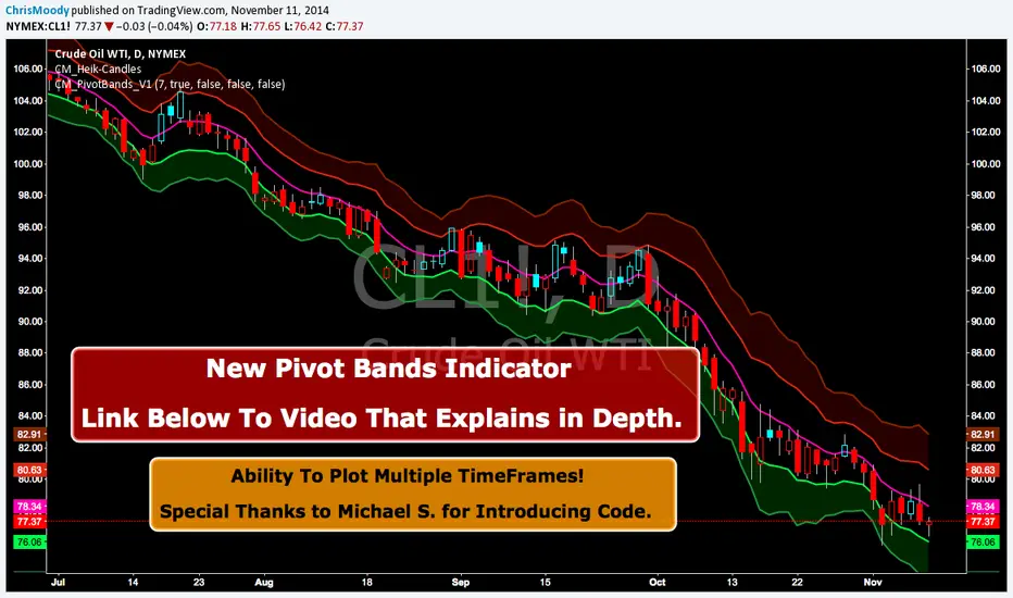
CM Pivot Bands V1CM_Pivot Bands V1
Special Thanks to Michael S for Introducing Code.
Instead of a Long Write Up I Recorded A Video Going Into Detail On V1 Of This Indicator. Please View To See My Initial Findings, My Thoughts For V2, And Items I Need YOUR Help With!!!
In Inputs Tab Indicator Has Ability to Turn On/Off Multiple TimeFrames…Thought Process Explained In Video.
Link To Video:
vimeopro.com
Link To PDF Mentioned In Video:
d.pr
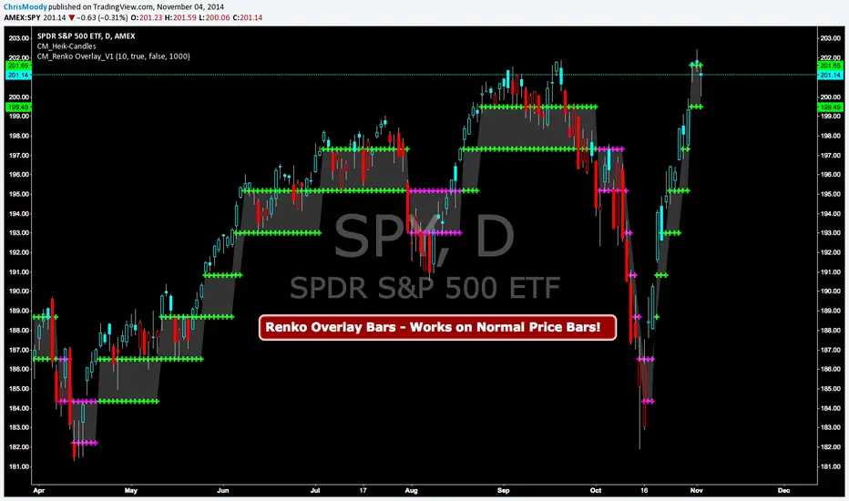
CM Renko Overlay BarsCM_Renko Overlay Bars V1
Overlays Renko Bars on Regular Price Bars.
Default Renko plot is based on Average True Range. Look Back period adjustable in Inputs Tab.
If you Choose to use "Traditional" Renko bars and pick the Size of the Renko Bars the please read below.
Value in Input Tab is multiplied by .001 (To work on Forex)
1 = 10 pips on EURUSD - 1 X .001 = .001 or 10 Pips
10 = .01 or 100 Pips
1000 = 1 point to the left of decimal. 1 Point in Stocks etc.
10000 = 10 Points on Stocks etc.
***V2 will fix this issue.
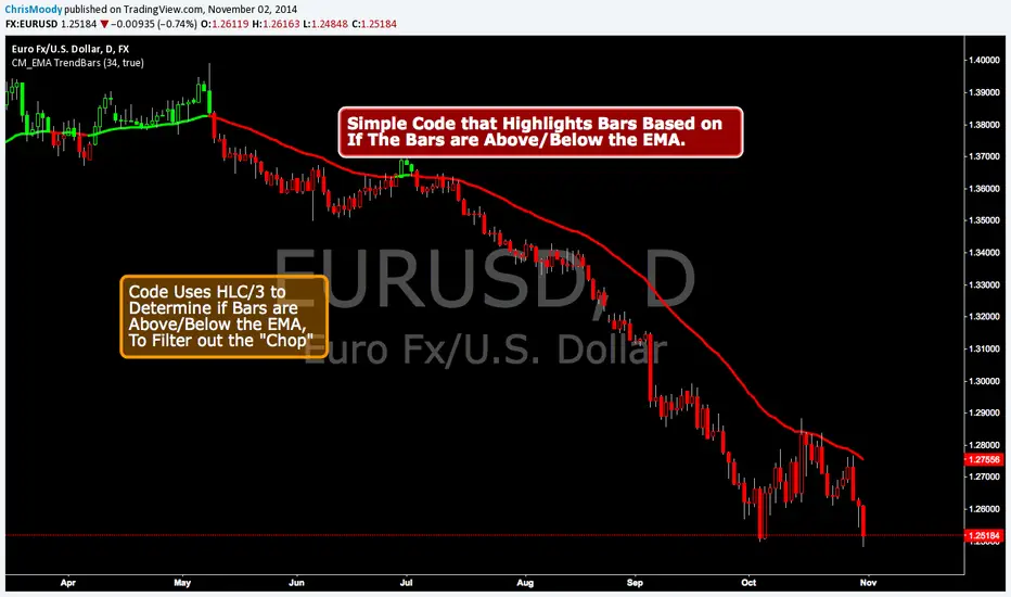
CM EMA Trend BarsThis Code Simply Changes the Bar Colors based on if the Bar is Above or Below the EMA.
Inputs via the Inputs Tab:
Ability to change the EMA Period.
Ability to Turn On/Off the EMA Plotted on the Screen
***Note - I used the HLC/3 To determine if the bar/candle is above or below the EMA. This Filters out the Chop and gets rid of many of the False Breaks above or below the EMA.
CM Enhanced Ichimoku Cloud V5Ichimoku Cloud Indicator With Cloud Shading Based On Trend!!!
I’m releasing this Indicator b/c of the New Feature that Allows Coding The Fill of The Cloud To Change Colors Based On Trend. However, I will be releasing a Much More Advanced Version Soon!!!
Current Features - Via Inputs Tab:
- Ability to Turn On/Off Every Plot Individually Via Check Box
- Ability To Turn On/Off Tenkan and Kinjun Crosses (Arrows)
***Features Coming Soon - All Will Have Capability to Turn On/Off:
- Bar Color Change when Entering The Cloud
- Filtered Tenkan and Kinjun Crosses To Plot Only With Trend, only Counter Trend, Or All Crosses
- Plot Arrows When Price Exits The Cloud.
- Plot Arrows When Lagging Line Crosses The Cloud Confirmed, or Not Confirmed by Price.
- Plus More!!!
- Basically Ability To Set Alerts Based On Any Condition!!!
WHAT ARE YOUR REQUESTS FOR FEATURES??? Comment Below.

CM Stochastic Multi-TimeFrameMulti TimeFrame Stochastic Loaded With Features.
Basics:
Ability to turn On/Off Crosses Only Above or Below High/Low Lines.
User sets Values Of High/Low lines.
Ability to turn On/Off All Crosses, Both BackGround Highlights and “B”, “S” Letters.
Ability to turn On/Off BackGround Highlights if Stoch is Above Or Below High/Low Lines.
Ability to All or Any Combination of these Features.
Multi Timeframe Capabilities:
Stoch defaults to current timeframe. You can change to many other timeframes.
Ability to turn On/Off Plotting 2nd Stoch on same TimeFrame with different settings
Ability to turn On/Off Plotting 2nd Stoch on Different TimeFrame
Much More…All Inputs and Options are Adjustable in Inputs Tab.

CM Willams %R and CCI BackGround HighlightCM_Willams %R and CCI BackGround Highlight
Created By User Request
Indicator Highlights:
Creates Red BackGround Highlight if CCI Or Williams %R are Above Upper Line (User Defined)
Creates Green BackGround Highlight if CCI Or Williams %R are Below Lower Line (User Defined)
Ability to Turn On/Off either Williams %R or CCI Highlights in Inputs Tab via Check Boxes.
Ability To Set All Parameters for CCI and Williams %R in Inputs Tab.
Ability to Set High/Low “Threshold” Lines for Both CCI and Williams %R in Inputs Tab.
***I was asked if you could plot Back Ground Highlights on Two Individual Indicators AND have it show if BOTH Indicators were Overbought and Oversold.
***The answer is Yes. On the Chart Above I have the same Shade of Red and Green for Both Indicators. However, you will notice when Both Indicators Show OverBought…Both Plot Red Back Ground Highlights Which = a Brighter Red. The same is True for Oversold Conditions. The Green Shows a Brighter Shade of Green.
***VERY IMPORTANT - It is difficult for a programmer to release Indicators with this feature because depending on what color background you use on your charts…THE COLORS LOOK COMPLETELY DIFFERENT. So If You Don’t Use The Black Back Ground Shown Above You Most Likely Will Need To Adjust The Transparency, and Possibly The Colors Themselves!!!!
Reference Page

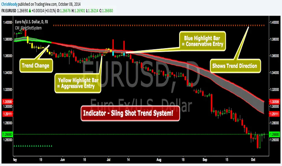
CM Sling Shot SystemSling Shot System + Even Better System.
I get this email about a Trend Following System that sells for $1000 but I could get it that day for only $500!!!
I watch the video showing this Amazing System which may have taken me an entire minute to figure out the code.
I code it up. And Hey…It’s not a bad system. It’s good for people who may need a Entry Signal to get them in a Trending Move, and KEEP them in a Trending Move while providing a defined Stop.
So I thought I would save the community the Very Fair price of Only $500 for a system that consists of a couple of EMA’s and a few Rules…and give it to you for free.
See Link Below for Main Chart Showing 2nd System!!!
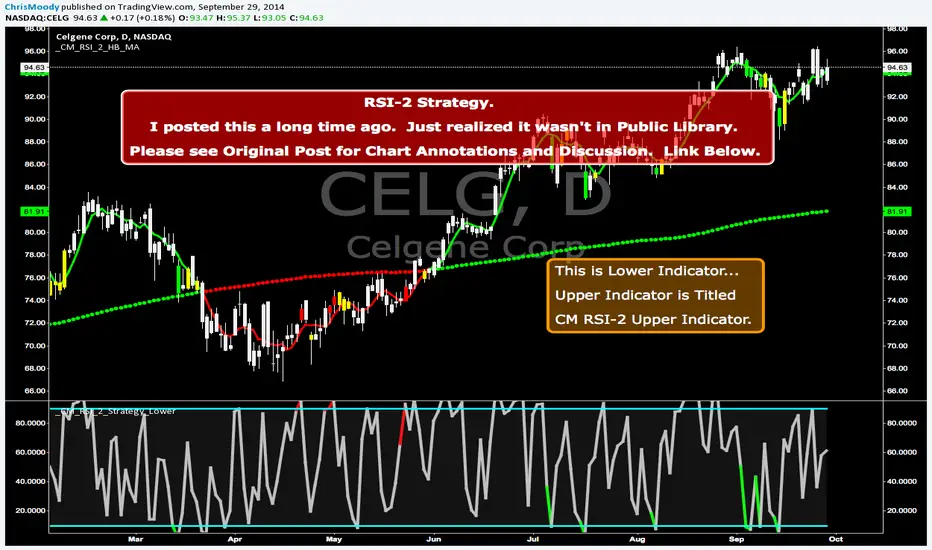
CM RSI-2 Strategy Lower IndicatorRSI-2 Strategy
***At the bottom of the page is a link where you can download the PDF of the Backtesting Results.
This year I am focusing on learning from two of the best mentors in the Industry with outstanding track records for Creating Systems, and learning the what methods actually work as far as back testing.
I came across the RSI-2 system that Larry Connors developed. Larry has become famous for his technical indicators, but his RSI-2 system is what actually put him “On The Map” per se. At first glance I didn’t think it would work well, but I decided to code it and ran backtests on the S&P 100 In Down Trending Markets, Up Trending Markets, and both combined. I was shocked by the results. So I thought I would provide them for you. I also ran a test on the Major forex Pairs (12) for the last 5 years, and All Forex Pairs (80) from 11/28/2007 - 6/09/2014, impressive results also.
The RSI-2 Strategy is designed to use on Daily Bars, however it is a short term trading strategy. The average length of time in a trade is just over 2 days. But the results CRUSH the general market averages.
Detailed Description of Indicators, Rules Below:
Link For PDF of Detailed Trade Results
d.pr
Original Post
CM RSI-2 Strategy - Upper Indicators.RSI-2 Strategy
***At the bottom of the page is a link where you can download the PDF of the Backtesting Results.
This year I am focusing on learning from two of the best mentors in the Industry with outstanding track records for Creating Systems, and learning the what methods actually work as far as back testing.
I came across the RSI-2 system that Larry Connors developed. Larry has become famous for his technical indicators, but his RSI-2 system is what actually put him “On The Map” per se. At first glance I didn’t think it would work well, but I decided to code it and ran backtests on the S&P 100 In Down Trending Markets, Up Trending Markets, and both combined. I was shocked by the results. So I thought I would provide them for you. I also ran a test on the Major forex Pairs (12) for the last 5 years, and All Forex Pairs (80) from 11/28/2007 - 6/09/2014, impressive results also.
The RSI-2 Strategy is designed to use on Daily Bars, however it is a short term trading strategy. The average length of time in a trade is just over 2 days. But the results CRUSH the general market averages.
Detailed Description of Indicators, Rules Below:
Link For PDF of Detailed Trade Results
d.pr
Original Post

CM Heikin-Ashi Candlesticks_V1Heikin-Ashi Paint Bars.
Paints Candlesticks or OHLC Bars The Exact Same as Traditional Heikin-Ashi Bars

Cryptocurrency Market Sentiment v1.0Introduction:
Capable of observing the market sentiment of the cryptocurrency market
The relative status of BTC and altcoins
How it works:
1. The general uptrend process of the cryptocurrency market is BTC → ETH → high-cap altcoins → low-cap altcoins. When funds cannot push up BTC's market cap, funds gradually flow into smaller-cap altcoins until the upward trend ends.
2. Select ETH as the representative of altcoins, and understand the sentiment and current stage
3. Mathematical principle : divide the price of ETH by the price of BTC, and then apply it to the RSI formula .
How to use it:
1. Similar to the RSI indicator , when CMS enters the overbought zone, it represents an active altcoin market, a passionate market sentiment , and the end of the uptrend.
2. When CMS enters the oversold zone, it indicates the leading stage of BTC in the rising trend or the capital flow back to BTC in the declining process .
3. If CMS is at a low level, long positions should focus on altcoins, and short positions should focus on BTC, and vice versa.
----------------------------------------------------------------------------------------------------------
简单介绍:
能够观察加密市场市场情绪
BTC和寨币的相对状态
如何工作:
1、加密市场一般的上涨过程为 BTC → ETH → 大市值山寨 → 小市值山寨,当资金无法推动大市值的BTC上涨时,资金就会逐渐流向市值较小的山寨,直到一轮上涨结束。
2、选取ETH作为altcoins的代表,通过ETH与BTC的关系来了解加密市场的情绪和目前上涨的阶段。
3、数学原理:将ETH的价格/BTC的价格,随后将其带入RSI公式
如何使用:
1、与RSI指标类似,当cms进入超买时,代表寨币市场的活跃,市场情绪热烈,上涨进入尾声。
2、当cms进入超卖时,为上涨中BTC领涨的阶段或下降过程中资金回流BTC。
3、如果cms在低位,做多应关注altcoins,做空应关注btc,反之亦然。

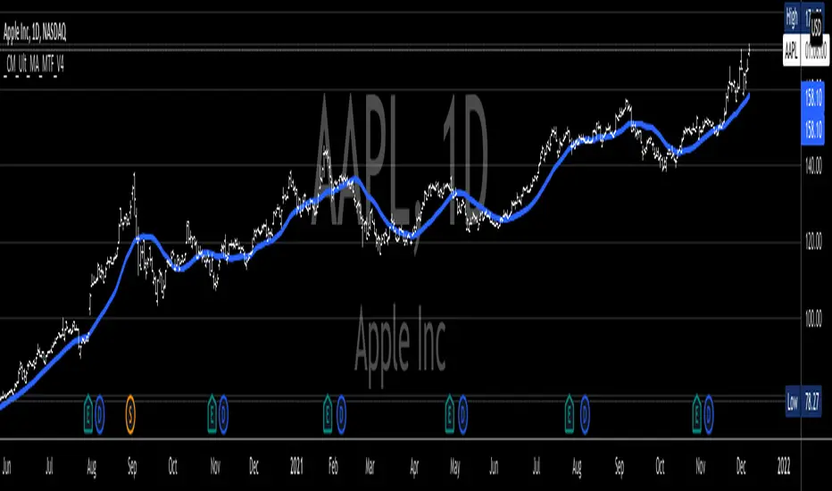
_CM_Ultimate_MA_MTF_V4***For a Detailed Video Overview Showing all of the Settings...
Click HERE to View Video
New _CM_Ultimate_MA_MTF_V4 - Update - 08-24-2021
Thanks to @SKTennis for help with code
Added Ability to Plot 1 or 2 Moving Averages - Fast MA & Slow MA
Added Ability to Plot Fast MA with Multi TimeFrame
Added Ability to Plot Slow MA with Multi TimeFrame
Added Ability to Color Fast MA Based on Slope of MA
Added Ability to Color Fast MA based on being Above/Below Slow MA
Added Ability to Plot 8 Types of Moving Averages
Simple, Exponential, Weighted, Hull, VWMA, RMA, TEMA, & Tilson T3
Added Ability to Set Alerts Based on:
Slope Change in the Fast MA Or Fast MA Crossing Above/Below Slow MA.
Added Ability to Plot "Fill" if Both Moving Averages are Turned ON
Added Ability to control Transparency of Fill
Added Alerts to Settings Pane.
Customized how Alerts work. Must keep Checked in Settings Pane, and When you go to Alerts Panel, Change Symbol to Indicator (_CM_Ultimate_MA_MTF_V4)
Customized Alerts to Show Symbol, TimeFrame, Closing Price, & Moving Average Signal Name in Alert
Alerts are Pre-Set to only Alert on Bar Close
See Video for Detailed Overview
New Updates Coming Soon!!!
***Please Post Feedback and Any Feature Requests in the Comments Section Below***
Klinger Oscillator AdvancedThe Klinger Oscillator is not fully implemented in Tradeview. While the description at de.tradingview.com is complete, the implementation is limited to the pure current volume movement. This results in no difference compared to the On Balance Volume indicator.
However, Klinger's goal was to incorporate the trend as volume force in its strength and duration into the calculation. The expression ((V x x T x 100)) for volume force only makes sense as an absolute value, which should probably be expressed as ((V x abs(2 x ((dm/cm) - 1)) x T x 100)). Additionally, there is a need to handle the theoretical possibility of cm == 0.
Since, in general, significantly more trading volume occurs at the closing price than during the day, an additional parameter for weighting the closing price is implemented. In intraday charts, considering the closing price, in my opinion, does not make sense.
The TradeView implementation is displayed on the chart for comparison. Particularly in the analysis of divergence, significant deviations become apparent.

Williams Vix Fix ultra complete indicator (Tartigradia)Williams VixFix is a realized volatility indicator developed by Larry Williams, and can help in finding market bottoms.
Indeed, as Williams describe in his paper, markets tend to find the lowest prices during times of highest volatility, which usually accompany times of highest fear. The VixFix is calculated as how much the current low price statistically deviates from the maximum within a given look-back period.
Although the VixFix originally only indicates market bottoms, its inverse may indicate market tops. As masa_crypto writes : "The inverse can be formulated by considering "how much the current high value statistically deviates from the minimum within a given look-back period." This transformation equates Vix_Fix_inverse. This indicator can be used for finding market tops, and therefore, is a good signal for a timing for taking a short position." However, in practice, the Inverse VixFix is much less reliable than the classical VixFix, but is nevertheless a good addition to get some additional context.
For more information on the Vix Fix, which is a strategy published under public domain:
* The VIX Fix, Larry Williams, Active Trader magazine, December 2007, web.archive.org
* Fixing the VIX: An Indicator to Beat Fear, Amber Hestla-Barnhart, Journal of Technical Analysis, March 13, 2015, ssrn.com
* Replicating the CBOE VIX using a synthetic volatility index trading algorithm, Dayne Cary and Gary van Vuuren, Cogent Economics & Finance, Volume 7, 2019, Issue 1, doi.org
Created By ChrisMoody on 12-26-2014...
V3 MAJOR Update on 1-05-2014
tista merged LazyBear's Black Dots filter in 2020:
Extended by Tartigradia in 10-2022:
* Can select a symbol different from current to calculate vixfix, allows to select SP:SPX to mimic the original VIX index.
* Inverse VixFix (from masa_crypto and web.archive.org)
* VixFix OHLC Bars plot
* Price / VixFix Candles plot (Pro Tip: draw trend lines to find good entry/exit points)
* Add ADX filtering, Minimaxis signals, Minimaxis filtering (from samgozman )
* Convert to pinescript v5
* Allow timeframe selection (MTF)
* Skip off days (more accurate reproduction of original VIX)
* Reorganized, cleaned up code, commented out parts, commented out or removed unused code (eg, some of the KC calculations)
* Changed default Bollinger Band settings to reduce false positives in crypto markets.
Set Index symbol to SPX, and index_current = false, and timeframe Weekly, to reproduce the original VIX as close as possible by the VIXFIX (use the Add Symbol option, because you want to plot CBOE:VIX on the same timeframe as the current chart, which may include extended session / weekends). With the Weekly timeframe, off days / extended session days should not change much, but with lower timeframes this is important, because nights and weekends can change how the graph appears and seemingly make them different because of timing misalignment when in reality they are not when properly aligned.

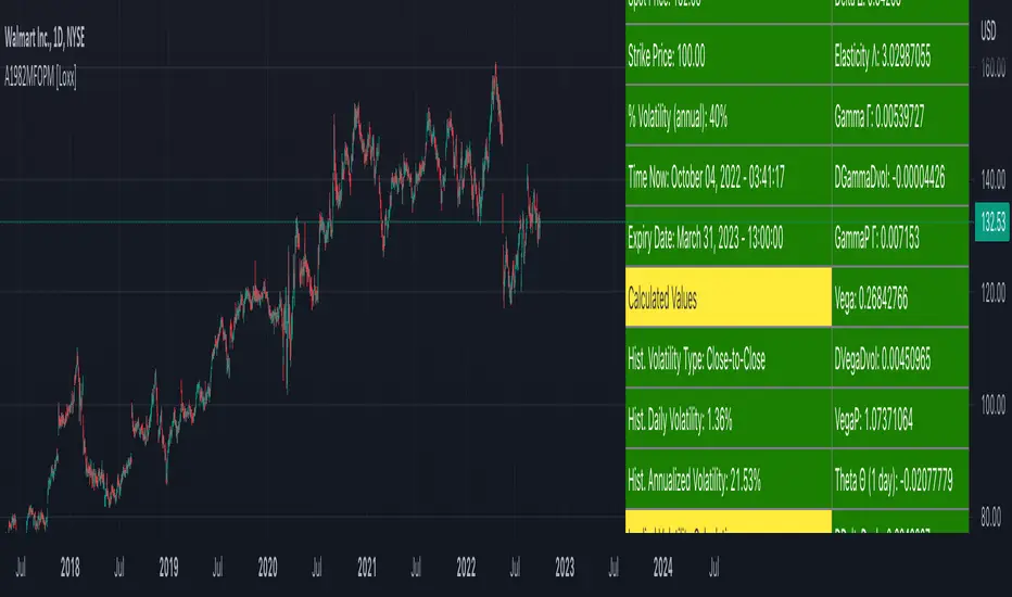
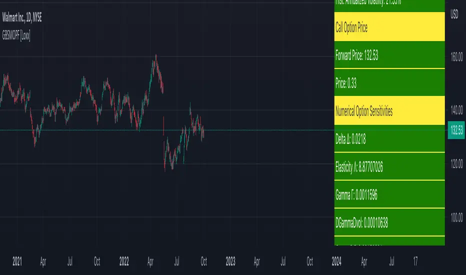
Asay (1982) Margined Futures Option Pricing Model [Loxx]Asay (1982) Margined Futures Option Pricing Model is an adaptation of the Black-Scholes-Merton Option Pricing Model including Analytical Greeks and implied volatility calculations. The following information is an excerpt from Espen Gaarder Haug's book "Option Pricing Formulas". This version is to price Options on Futures where premium is fully margined. This means the Risk-free Rate, dividend, and cost to carry are all zero. The options sensitivities (Greeks) are the partial derivatives of the Black-Scholes-Merton ( BSM ) formula. Analytical Greeks for our purposes here are broken down into various categories:
Delta Greeks: Delta, DDeltaDvol, Elasticity
Gamma Greeks: Gamma, GammaP, DGammaDvol, Speed
Vega Greeks: Vega , DVegaDvol/Vomma, VegaP
Theta Greeks: Theta
Probability Greeks: StrikeDelta, Risk Neutral Density
(See the code for more details)
Black-Scholes-Merton Option Pricing
The Black-Scholes-Merton model can be "generalized" by incorporating a cost-of-carry rate b. This model can be used to price European options on stocks, stocks paying a continuous dividend yield, options on futures , and currency options:
c = S * e^((b - r) * T) * N(d1) - X * e^(-r * T) * N(d2)
p = X * e^(-r * T) * N(-d2) - S * e^((b - r) * T) * N(-d1)
where
d1 = (log(S / X) + (b + v^2 / 2) * T) / (v * T^0.5)
d2 = d1 - v * T^0.5
b = r ... gives the Black and Scholes (1973) stock option model.
b = r — q ... gives the Merton (1973) stock option model with continuous dividend yield q.
b = 0 ... gives the Black (1976) futures option model.
b = 0 and r = 0 ... gives the Asay (1982) margined futures option model. <== this is the one used for this indicator!
b = r — rf ... gives the Garman and Kohlhagen (1983) currency option model.
Inputs
S = Stock price.
X = Strike price of option.
T = Time to expiration in years.
r = Risk-free rate
d = dividend yield
v = Volatility of the underlying asset price
cnd (x) = The cumulative normal distribution function
nd(x) = The standard normal density function
convertingToCCRate(r, cmp ) = Rate compounder
gImpliedVolatilityNR(string CallPutFlag, float S, float x, float T, float r, float b, float cm , float epsilon) = Implied volatility via Newton Raphson
gBlackScholesImpVolBisection(string CallPutFlag, float S, float x, float T, float r, float b, float cm ) = implied volatility via bisection
Implied Volatility: The Bisection Method
The Newton-Raphson method requires knowledge of the partial derivative of the option pricing formula with respect to volatility ( vega ) when searching for the implied volatility . For some options (exotic and American options in particular), vega is not known analytically. The bisection method is an even simpler method to estimate implied volatility when vega is unknown. The bisection method requires two initial volatility estimates (seed values):
1. A "low" estimate of the implied volatility , al, corresponding to an option value, CL
2. A "high" volatility estimate, aH, corresponding to an option value, CH
The option market price, Cm , lies between CL and cH . The bisection estimate is given as the linear interpolation between the two estimates:
v(i + 1) = v(L) + (c(m) - c(L)) * (v(H) - v(L)) / (c(H) - c(L))
Replace v(L) with v(i + 1) if c(v(i + 1)) < c(m), or else replace v(H) with v(i + 1) if c(v(i + 1)) > c(m) until |c(m) - c(v(i + 1))| <= E, at which point v(i + 1) is the implied volatility and E is the desired degree of accuracy.
Implied Volatility: Newton-Raphson Method
The Newton-Raphson method is an efficient way to find the implied volatility of an option contract. It is nothing more than a simple iteration technique for solving one-dimensional nonlinear equations (any introductory textbook in calculus will offer an intuitive explanation). The method seldom uses more than two to three iterations before it converges to the implied volatility . Let
v(i + 1) = v(i) + (c(v(i)) - c(m)) / (dc / dv (i))
until |c(m) - c(v(i + 1))| <= E at which point v(i + 1) is the implied volatility , E is the desired degree of accuracy, c(m) is the market price of the option, and dc/ dv (i) is the vega of the option evaluaated at v(i) (the sensitivity of the option value for a small change in volatility ).
Things to know
Only works on the daily timeframe and for the current source price.
You can adjust the text size to fit the screen
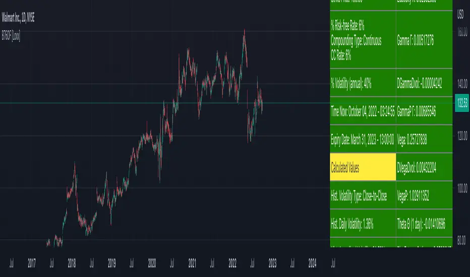
Black-76 Options on Futures [Loxx]Black-76 Options on Futures is an adaptation of the Black-Scholes-Merton Option Pricing Model including Analytical Greeks and implied volatility calculations. The following information is an excerpt from Espen Gaarder Haug's book "Option Pricing Formulas". This version is to price Options on Futures. The options sensitivities (Greeks) are the partial derivatives of the Black-Scholes-Merton ( BSM ) formula. Analytical Greeks for our purposes here are broken down into various categories:
Delta Greeks: Delta, DDeltaDvol, Elasticity
Gamma Greeks: Gamma, GammaP, DGammaDvol, Speed
Vega Greeks: Vega , DVegaDvol/Vomma, VegaP
Theta Greeks: Theta
Rate/Carry Greeks: Rho futures option
Probability Greeks: StrikeDelta, Risk Neutral Density
(See the code for more details)
Black-Scholes-Merton Option Pricing
The Black-Scholes-Merton model can be "generalized" by incorporating a cost-of-carry rate b. This model can be used to price European options on stocks, stocks paying a continuous dividend yield, options on futures , and currency options:
c = S * e^((b - r) * T) * N(d1) - X * e^(-r * T) * N(d2)
p = X * e^(-r * T) * N(-d2) - S * e^((b - r) * T) * N(-d1)
where
d1 = (log(S / X) + (b + v^2 / 2) * T) / (v * T^0.5)
d2 = d1 - v * T^0.5
b = r ... gives the Black and Scholes (1973) stock option model.
b = r — q ... gives the Merton (1973) stock option model with continuous dividend yield q.
b = 0 ... gives the Black (1976) futures option model. <== this is the one used for this indicator!
b = 0 and r = 0 ... gives the Asay (1982) margined futures option model.
b = r — rf ... gives the Garman and Kohlhagen (1983) currency option model.
Inputs
S = Stock price.
X = Strike price of option.
T = Time to expiration in years.
r = Risk-free rate
d = dividend yield
v = Volatility of the underlying asset price
cnd (x) = The cumulative normal distribution function
nd(x) = The standard normal density function
convertingToCCRate(r, cmp ) = Rate compounder
gImpliedVolatilityNR(string CallPutFlag, float S, float x, float T, float r, float b, float cm , float epsilon) = Implied volatility via Newton Raphson
gBlackScholesImpVolBisection(string CallPutFlag, float S, float x, float T, float r, float b, float cm ) = implied volatility via bisection
Implied Volatility: The Bisection Method
The Newton-Raphson method requires knowledge of the partial derivative of the option pricing formula with respect to volatility ( vega ) when searching for the implied volatility . For some options (exotic and American options in particular), vega is not known analytically. The bisection method is an even simpler method to estimate implied volatility when vega is unknown. The bisection method requires two initial volatility estimates (seed values):
1. A "low" estimate of the implied volatility , al, corresponding to an option value, CL
2. A "high" volatility estimate, aH, corresponding to an option value, CH
The option market price, Cm , lies between CL and cH . The bisection estimate is given as the linear interpolation between the two estimates:
v(i + 1) = v(L) + (c(m) - c(L)) * (v(H) - v(L)) / (c(H) - c(L))
Replace v(L) with v(i + 1) if c(v(i + 1)) < c(m), or else replace v(H) with v(i + 1) if c(v(i + 1)) > c(m) until |c(m) - c(v(i + 1))| <= E, at which point v(i + 1) is the implied volatility and E is the desired degree of accuracy.
Implied Volatility: Newton-Raphson Method
The Newton-Raphson method is an efficient way to find the implied volatility of an option contract. It is nothing more than a simple iteration technique for solving one-dimensional nonlinear equations (any introductory textbook in calculus will offer an intuitive explanation). The method seldom uses more than two to three iterations before it converges to the implied volatility . Let
v(i + 1) = v(i) + (c(v(i)) - c(m)) / (dc / dv (i))
until |c(m) - c(v(i + 1))| <= E at which point v(i + 1) is the implied volatility , E is the desired degree of accuracy, c(m) is the market price of the option, and dc/ dv (i) is the vega of the option evaluaated at v(i) (the sensitivity of the option value for a small change in volatility ).
Things to know
Only works on the daily timeframe and for the current source price.
You can adjust the text size to fit the screen
Garman and Kohlhagen (1983) for Currency Options [Loxx]Garman and Kohlhagen (1983) for Currency Options is an adaptation of the Black-Scholes-Merton Option Pricing Model including Analytical Greeks and implied volatility calculations. The following information is an excerpt from Espen Gaarder Haug's book "Option Pricing Formulas". This version of BSMOPM is to price Currency Options. The options sensitivities (Greeks) are the partial derivatives of the Black-Scholes-Merton ( BSM ) formula. Analytical Greeks for our purposes here are broken down into various categories:
Delta Greeks: Delta, DDeltaDvol, Elasticity
Gamma Greeks: Gamma, GammaP, DGammaDSpot/speed, DGammaDvol/Zomma
Vega Greeks: Vega , DVegaDvol/Vomma, VegaP, Speed
Theta Greeks: Theta
Rate/Carry Greeks: Rho, Rho futures option, Carry Rho, Phi/Rho2
Probability Greeks: StrikeDelta, Risk Neutral Density
(See the code for more details)
Black-Scholes-Merton Option Pricing for Currency Options
The Garman and Kohlhagen (1983) modified Black-Scholes model can be used to price European currency options; see also Grabbe (1983). The model is mathematically equivalent to the Merton (1973) model presented earlier. The only difference is that the dividend yield is replaced by the risk-free rate of the foreign currency rf:
c = S * e^(-rf * T) * N(d1) - X * e^(-r * T) * N(d2)
p = X * e^(-r * T) * N(-d2) - S * e^(-rf * T) * N(-d1)
where
d1 = (log(S / X) + (r - rf + v^2 / 2) * T) / (v * T^0.5)
d2 = d1 - v * T^0.5
For more information on currency options, see DeRosa (2000)
Inputs
S = Stock price.
X = Strike price of option.
T = Time to expiration in years.
r = Risk-free rate
rf = Risk-free rate of the foreign currency
v = Volatility of the underlying asset price
cnd (x) = The cumulative normal distribution function
nd(x) = The standard normal density function
convertingToCCRate(r, cmp ) = Rate compounder
gImpliedVolatilityNR(string CallPutFlag, float S, float x, float T, float r, float b, float cm , float epsilon) = Implied volatility via Newton Raphson
gBlackScholesImpVolBisection(string CallPutFlag, float S, float x, float T, float r, float b, float cm ) = implied volatility via bisection
Implied Volatility: The Bisection Method
The Newton-Raphson method requires knowledge of the partial derivative of the option pricing formula with respect to volatility ( vega ) when searching for the implied volatility . For some options (exotic and American options in particular), vega is not known analytically. The bisection method is an even simpler method to estimate implied volatility when vega is unknown. The bisection method requires two initial volatility estimates (seed values):
1. A "low" estimate of the implied volatility , al, corresponding to an option value, CL
2. A "high" volatility estimate, aH, corresponding to an option value, CH
The option market price, Cm , lies between CL and cH . The bisection estimate is given as the linear interpolation between the two estimates:
v(i + 1) = v(L) + (c(m) - c(L)) * (v(H) - v(L)) / (c(H) - c(L))
Replace v(L) with v(i + 1) if c(v(i + 1)) < c(m), or else replace v(H) with v(i + 1) if c(v(i + 1)) > c(m) until |c(m) - c(v(i + 1))| <= E, at which point v(i + 1) is the implied volatility and E is the desired degree of accuracy.
Implied Volatility: Newton-Raphson Method
The Newton-Raphson method is an efficient way to find the implied volatility of an option contract. It is nothing more than a simple iteration technique for solving one-dimensional nonlinear equations (any introductory textbook in calculus will offer an intuitive explanation). The method seldom uses more than two to three iterations before it converges to the implied volatility . Let
v(i + 1) = v(i) + (c(v(i)) - c(m)) / (dc / dv (i))
until |c(m) - c(v(i + 1))| <= E at which point v(i + 1) is the implied volatility , E is the desired degree of accuracy, c(m) is the market price of the option, and dc/ dv (i) is the vega of the option evaluaated at v(i) (the sensitivity of the option value for a small change in volatility ).
Things to know
Only works on the daily timeframe and for the current source price.
You can adjust the text size to fit the screen
Related indicators:
BSM OPM 1973 w/ Continuous Dividend Yield
Black-Scholes 1973 OPM on Non-Dividend Paying Stocks
Generalized Black-Scholes-Merton w/ Analytical Greeks
Generalized Black-Scholes-Merton Option Pricing Formula
Sprenkle 1964 Option Pricing Model w/ Num. Greeks
Modified Bachelier Option Pricing Model w/ Num. Greeks
Bachelier 1900 Option Pricing Model w/ Numerical Greeks

BSM OPM 1973 w/ Continuous Dividend Yield [Loxx]Generalized Black-Scholes-Merton w/ Analytical Greeks is an adaptation of the Black-Scholes-Merton Option Pricing Model including Analytical Greeks and implied volatility calculations. The following information is an excerpt from Espen Gaarder Haug's book "Option Pricing Formulas". The options sensitivities (Greeks) are the partial derivatives of the Black-Scholes-Merton ( BSM ) formula. Analytical Greeks for our purposes here are broken down into various categories:
Delta Greeks: Delta, DDeltaDvol, Elasticity
Gamma Greeks: Gamma, GammaP, DGammaDSpot/speed, DGammaDvol/Zomma
Vega Greeks: Vega , DVegaDvol/Vomma, VegaP
Theta Greeks: Theta
Rate/Carry Greeks: Rho, Rho futures option, Carry Rho, Phi/Rho2
Probability Greeks: StrikeDelta, Risk Neutral Density
(See the code for more details)
Black-Scholes-Merton Option Pricing
The Black-Scholes-Merton model can be "generalized" by incorporating a cost-of-carry rate b. This model can be used to price European options on stocks, stocks paying a continuous dividend yield, options on futures, and currency options:
c = S * e^((b - r) * T) * N(d1) - X * e^(-r * T) * N(d2)
p = X * e^(-r * T) * N(-d2) - S * e^((b - r) * T) * N(-d1)
where
d1 = (log(S / X) + (b + v^2 / 2) * T) / (v * T^0.5)
d2 = d1 - v * T^0.5
b = r ... gives the Black and Scholes (1973) stock option model.
b = r — q ... gives the Merton (1973) stock option model with continuous dividend yield q. <== this is the one used for this indicator!
b = 0 ... gives the Black (1976) futures option model.
b = 0 and r = 0 ... gives the Asay (1982) margined futures option model.
b = r — rf ... gives the Garman and Kohlhagen (1983) currency option model.
Inputs
S = Stock price.
X = Strike price of option.
T = Time to expiration in years.
r = Risk-free rate
d = dividend yield
v = Volatility of the underlying asset price
cnd (x) = The cumulative normal distribution function
nd(x) = The standard normal density function
convertingToCCRate(r, cmp ) = Rate compounder
gImpliedVolatilityNR(string CallPutFlag, float S, float x, float T, float r, float b, float cm , float epsilon) = Implied volatility via Newton Raphson
gBlackScholesImpVolBisection(string CallPutFlag, float S, float x, float T, float r, float b, float cm ) = implied volatility via bisection
Implied Volatility: The Bisection Method
The Newton-Raphson method requires knowledge of the partial derivative of the option pricing formula with respect to volatility ( vega ) when searching for the implied volatility . For some options (exotic and American options in particular), vega is not known analytically. The bisection method is an even simpler method to estimate implied volatility when vega is unknown. The bisection method requires two initial volatility estimates (seed values):
1. A "low" estimate of the implied volatility , al, corresponding to an option value, CL
2. A "high" volatility estimate, aH, corresponding to an option value, CH
The option market price, Cm , lies between CL and cH . The bisection estimate is given as the linear interpolation between the two estimates:
v(i + 1) = v(L) + (c(m) - c(L)) * (v(H) - v(L)) / (c(H) - c(L))
Replace v(L) with v(i + 1) if c(v(i + 1)) < c(m), or else replace v(H) with v(i + 1) if c(v(i + 1)) > c(m) until |c(m) - c(v(i + 1))| <= E, at which point v(i + 1) is the implied volatility and E is the desired degree of accuracy.
Implied Volatility: Newton-Raphson Method
The Newton-Raphson method is an efficient way to find the implied volatility of an option contract. It is nothing more than a simple iteration technique for solving one-dimensional nonlinear equations (any introductory textbook in calculus will offer an intuitive explanation). The method seldom uses more than two to three iterations before it converges to the implied volatility . Let
v(i + 1) = v(i) + (c(v(i)) - c(m)) / (dc / dv (i))
until |c(m) - c(v(i + 1))| <= E at which point v(i + 1) is the implied volatility , E is the desired degree of accuracy, c(m) is the market price of the option, and dc/ dv (i) is the vega of the option evaluaated at v(i) (the sensitivity of the option value for a small change in volatility ).
Things to know
Only works on the daily timeframe and for the current source price.
You can adjust the text size to fit the screen

Black-Scholes 1973 OPM on Non-Dividend Paying Stocks [Loxx]Black-Scholes 1973 OPM on Non-Dividend Paying Stocks is an adaptation of the Black-Scholes-Merton Option Pricing Model including Analytical Greeks and implied volatility calculations. Making b equal to r yields the BSM model where dividends are not considered. The following information is an excerpt from Espen Gaarder Haug's book "Option Pricing Formulas". The options sensitivities (Greeks) are the partial derivatives of the Black-Scholes-Merton ( BSM ) formula. For our purposes here are, Analytical Greeks are broken down into various categories:
Delta Greeks: Delta, DDeltaDvol, Elasticity
Gamma Greeks: Gamma, GammaP, DGammaDSpot/speed, DGammaDvol/Zomma
Vega Greeks: Vega , DVegaDvol/Vomma, VegaP
Theta Greeks: Theta
Rate/Carry Greeks: Rho
Probability Greeks: StrikeDelta, Risk Neutral Density
(See the code for more details)
Black-Scholes-Merton Option Pricing
The BSM formula and its binomial counterpart may easily be the most used "probability model/tool" in everyday use — even if we con- sider all other scientific disciplines. Literally tens of thousands of people, including traders, market makers, and salespeople, use option formulas several times a day. Hardly any other area has seen such dramatic growth as the options and derivatives businesses. In this chapter we look at the various versions of the basic option formula. In 1997 Myron Scholes and Robert Merton were awarded the Nobel Prize (The Bank of Sweden Prize in Economic Sciences in Memory of Alfred Nobel). Unfortunately, Fischer Black died of cancer in 1995 before he also would have received the prize.
It is worth mentioning that it was not the option formula itself that Myron Scholes and Robert Merton were awarded the Nobel Prize for, the formula was actually already invented, but rather for the way they derived it — the replicating portfolio argument, continuous- time dynamic delta hedging, as well as making the formula consistent with the capital asset pricing model (CAPM). The continuous dynamic replication argument is unfortunately far from robust. The popularity among traders for using option formulas heavily relies on hedging options with options and on the top of this dynamic delta hedging, see Higgins (1902), Nelson (1904), Mello and Neuhaus (1998), Derman and Taleb (2005), as well as Haug (2006) for more details on this topic. In any case, this book is about option formulas and not so much about how to derive them.
Provided here are the various versions of the Black-Scholes-Merton formula presented in the literature. All formulas in this section are originally derived based on the underlying asset S follows a geometric Brownian motion
dS = mu * S * dt + v * S * dz
where t is the expected instantaneous rate of return on the underlying asset, a is the instantaneous volatility of the rate of return, and dz is a Wiener process.
The formula derived by Black and Scholes (1973) can be used to value a European option on a stock that does not pay dividends before the option's expiration date. Letting c and p denote the price of European call and put options, respectively, the formula states that
c = S * N(d1) - X * e^(-r * T) * N(d2)
p = X * e^(-r * T) * N(d2) - S * N(d1)
where
d1 = (log(S / X) + (r + v^2 / 2) * T) / (v * T^0.5)
d2 = (log(S / X) + (r - v^2 / 2) * T) / (v * T^0.5) = d1 - v * T^0.5
**This version of the Black-Scholes formula can also be used to price American call options on a non-dividend-paying stock, since it will never be optimal to exercise the option before expiration.**
Inputs
S = Stock price.
X = Strike price of option.
T = Time to expiration in years.
r = Risk-free rate
b = Cost of carry
v = Volatility of the underlying asset price
cnd (x) = The cumulative normal distribution function
nd(x) = The standard normal density function
convertingToCCRate(r, cmp ) = Rate compounder
gImpliedVolatilityNR(string CallPutFlag, float S, float x, float T, float r, float b, float cm , float epsilon) = Implied volatility via Newton Raphson
gBlackScholesImpVolBisection(string CallPutFlag, float S, float x, float T, float r, float b, float cm ) = implied volatility via bisection
Implied Volatility: The Bisection Method
The Newton-Raphson method requires knowledge of the partial derivative of the option pricing formula with respect to volatility ( vega ) when searching for the implied volatility . For some options (exotic and American options in particular), vega is not known analytically. The bisection method is an even simpler method to estimate implied volatility when vega is unknown. The bisection method requires two initial volatility estimates (seed values):
1. A "low" estimate of the implied volatility , al, corresponding to an option value, CL
2. A "high" volatility estimate, aH, corresponding to an option value, CH
The option market price, Cm , lies between CL and cH . The bisection estimate is given as the linear interpolation between the two estimates:
v(i + 1) = v(L) + (c(m) - c(L)) * (v(H) - v(L)) / (c(H) - c(L))
Replace v(L) with v(i + 1) if c(v(i + 1)) < c(m), or else replace v(H) with v(i + 1) if c(v(i + 1)) > c(m) until |c(m) - c(v(i + 1))| <= E, at which point v(i + 1) is the implied volatility and E is the desired degree of accuracy.
Implied Volatility: Newton-Raphson Method
The Newton-Raphson method is an efficient way to find the implied volatility of an option contract. It is nothing more than a simple iteration technique for solving one-dimensional nonlinear equations (any introductory textbook in calculus will offer an intuitive explanation). The method seldom uses more than two to three iterations before it converges to the implied volatility . Let
v(i + 1) = v(i) + (c(v(i)) - c(m)) / (dc / dv (i))
until |c(m) - c(v(i + 1))| <= E at which point v(i + 1) is the implied volatility , E is the desired degree of accuracy, c(m) is the market price of the option, and dc/ dv (i) is the vega of the option evaluaated at v(i) (the sensitivity of the option value for a small change in volatility ).
Things to know
Only works on the daily timeframe and for the current source price.
You can adjust the text size to fit the screen

Generalized Black-Scholes-Merton w/ Analytical Greeks [Loxx]Generalized Black-Scholes-Merton w/ Analytical Greeks is an adaptation of the Black-Scholes-Merton Option Pricing Model including Analytical Greeks and implied volatility calculations. The following information is an excerpt from Espen Gaarder Haug's book "Option Pricing Formulas". The options sensitivities (Greeks) are the partial derivatives of the Black-Scholes-Merton (BSM) formula. Analytical Greeks for our purposes here are broken down into various categories:
Delta Greeks: Delta, DDeltaDvol, Elasticity
Gamma Greeks: Gamma, GammaP, DGammaDSpot/speed, DGammaDvol/Zomma
Vega Greeks: Vega, DVegaDvol/Vomma, VegaP
Theta Greeks: Theta
Rate/Carry Greeks: Rho, Rho futures option, Carry Rho, Phi/Rho2
Probability Greeks: StrikeDelta, Risk Neutral Density
(See the code for more details)
Black-Scholes-Merton Option Pricing
The BSM formula and its binomial counterpart may easily be the most used "probability model/tool" in everyday use — even if we con- sider all other scientific disciplines. Literally tens of thousands of people, including traders, market makers, and salespeople, use option formulas several times a day. Hardly any other area has seen such dramatic growth as the options and derivatives businesses. In this chapter we look at the various versions of the basic option formula. In 1997 Myron Scholes and Robert Merton were awarded the Nobel Prize (The Bank of Sweden Prize in Economic Sciences in Memory of Alfred Nobel). Unfortunately, Fischer Black died of cancer in 1995 before he also would have received the prize.
It is worth mentioning that it was not the option formula itself that Myron Scholes and Robert Merton were awarded the Nobel Prize for, the formula was actually already invented, but rather for the way they derived it — the replicating portfolio argument, continuous- time dynamic delta hedging, as well as making the formula consistent with the capital asset pricing model (CAPM). The continuous dynamic replication argument is unfortunately far from robust. The popularity among traders for using option formulas heavily relies on hedging options with options and on the top of this dynamic delta hedging, see Higgins (1902), Nelson (1904), Mello and Neuhaus (1998), Derman and Taleb (2005), as well as Haug (2006) for more details on this topic. In any case, this book is about option formulas and not so much about how to derive them.
Provided here are the various versions of the Black-Scholes-Merton formula presented in the literature. All formulas in this section are originally derived based on the underlying asset S follows a geometric Brownian motion
dS = mu * S * dt + v * S * dz
where t is the expected instantaneous rate of return on the underlying asset, a is the instantaneous volatility of the rate of return, and dz is a Wiener process.
The formula derived by Black and Scholes (1973) can be used to value a European option on a stock that does not pay dividends before the option's expiration date. Letting c and p denote the price of European call and put options, respectively, the formula states that
c = S * N(d1) - X * e^(-r * T) * N(d2)
p = X * e^(-r * T) * N(d2) - S * N(d1)
where
d1 = (log(S / X) + (r + v^2 / 2) * T) / (v * T^0.5)
d2 = (log(S / X) + (r - v^2 / 2) * T) / (v * T^0.5) = d1 - v * T^0.5
Inputs
S = Stock price.
X = Strike price of option.
T = Time to expiration in years.
r = Risk-free rate
b = Cost of carry
v = Volatility of the underlying asset price
cnd (x) = The cumulative normal distribution function
nd(x) = The standard normal density function
convertingToCCRate(r, cmp ) = Rate compounder
gImpliedVolatilityNR(string CallPutFlag, float S, float x, float T, float r, float b, float cm , float epsilon) = Implied volatility via Newton Raphson
gBlackScholesImpVolBisection(string CallPutFlag, float S, float x, float T, float r, float b, float cm ) = implied volatility via bisection
Implied Volatility: The Bisection Method
The Newton-Raphson method requires knowledge of the partial derivative of the option pricing formula with respect to volatility ( vega ) when searching for the implied volatility . For some options (exotic and American options in particular), vega is not known analytically. The bisection method is an even simpler method to estimate implied volatility when vega is unknown. The bisection method requires two initial volatility estimates (seed values):
1. A "low" estimate of the implied volatility , al, corresponding to an option value, CL
2. A "high" volatility estimate, aH, corresponding to an option value, CH
The option market price, Cm , lies between CL and cH . The bisection estimate is given as the linear interpolation between the two estimates:
v(i + 1) = v(L) + (c(m) - c(L)) * (v(H) - v(L)) / (c(H) - c(L))
Replace v(L) with v(i + 1) if c(v(i + 1)) < c(m), or else replace v(H) with v(i + 1) if c(v(i + 1)) > c(m) until |c(m) - c(v(i + 1))| <= E, at which point v(i + 1) is the implied volatility and E is the desired degree of accuracy.
Implied Volatility: Newton-Raphson Method
The Newton-Raphson method is an efficient way to find the implied volatility of an option contract. It is nothing more than a simple iteration technique for solving one-dimensional nonlinear equations (any introductory textbook in calculus will offer an intuitive explanation). The method seldom uses more than two to three iterations before it converges to the implied volatility . Let
v(i + 1) = v(i) + (c(v(i)) - c(m)) / (dc / dv (i))
until |c(m) - c(v(i + 1))| <= E at which point v(i + 1) is the implied volatility , E is the desired degree of accuracy, c(m) is the market price of the option, and dc/ dv (i) is the vega of the option evaluaated at v(i) (the sensitivity of the option value for a small change in volatility ).
Things to know
Only works on the daily timeframe and for the current source price.
You can adjust the text size to fit the screen

Generalized Black-Scholes-Merton Option Pricing Formula [Loxx]Generalized Black-Scholes-Merton Option Pricing Formula is an adaptation of the Black-Scholes-Merton Option Pricing Model including Numerical Greeks aka "Option Sensitivities" and implied volatility calculations. The following information is an excerpt from Espen Gaarder Haug's book "Option Pricing Formulas".
Black-Scholes-Merton Option Pricing
The BSM formula and its binomial counterpart may easily be the most used "probability model/tool" in everyday use — even if we con- sider all other scientific disciplines. Literally tens of thousands of people, including traders, market makers, and salespeople, use option formulas several times a day. Hardly any other area has seen such dramatic growth as the options and derivatives businesses. In this chapter we look at the various versions of the basic option formula. In 1997 Myron Scholes and Robert Merton were awarded the Nobel Prize (The Bank of Sweden Prize in Economic Sciences in Memory of Alfred Nobel). Unfortunately, Fischer Black died of cancer in 1995 before he also would have received the prize.
It is worth mentioning that it was not the option formula itself that Myron Scholes and Robert Merton were awarded the Nobel Prize for, the formula was actually already invented, but rather for the way they derived it — the replicating portfolio argument, continuous- time dynamic delta hedging, as well as making the formula consistent with the capital asset pricing model (CAPM). The continuous dynamic replication argument is unfortunately far from robust. The popularity among traders for using option formulas heavily relies on hedging options with options and on the top of this dynamic delta hedging, see Higgins (1902), Nelson (1904), Mello and Neuhaus (1998), Derman and Taleb (2005), as well as Haug (2006) for more details on this topic. In any case, this book is about option formulas and not so much about how to derive them.
Provided here are the various versions of the Black-Scholes-Merton formula presented in the literature. All formulas in this section are originally derived based on the underlying asset S follows a geometric Brownian motion
dS = mu * S * dt + v * S * dz
where t is the expected instantaneous rate of return on the underlying asset, a is the instantaneous volatility of the rate of return, and dz is a Wiener process.
The formula derived by Black and Scholes (1973) can be used to value a European option on a stock that does not pay dividends before the option's expiration date. Letting c and p denote the price of European call and put options, respectively, the formula states that
c = S * N(d1) - X * e^(-r * T) * N(d2)
p = X * e^(-r * T) * N(d2) - S * N(d1)
where
d1 = (log(S / X) + (r + v^2 / 2) * T) / (v * T^0.5)
d2 = (log(S / X) + (r - v^2 / 2) * T) / (v * T^0.5) = d1 - v * T^0.5
Inputs
S = Stock price.
X = Strike price of option.
T = Time to expiration in years.
r = Risk-free rate
b = Cost of carry
v = Volatility of the underlying asset price
cnd (x) = The cumulative normal distribution function
nd(x) = The standard normal density function
convertingToCCRate(r, cmp ) = Rate compounder
gImpliedVolatilityNR(string CallPutFlag, float S, float x, float T, float r, float b, float cm, float epsilon) = Implied volatility via Newton Raphson
gBlackScholesImpVolBisection(string CallPutFlag, float S, float x, float T, float r, float b, float cm) = implied volatility via bisection
Implied Volatility: The Bisection Method
The Newton-Raphson method requires knowledge of the partial derivative of the option pricing formula with respect to volatility (vega) when searching for the implied volatility. For some options (exotic and American options in particular), vega is not known analytically. The bisection method is an even simpler method to estimate implied volatility when vega is unknown. The bisection method requires two initial volatility estimates (seed values):
1. A "low" estimate of the implied volatility, al, corresponding to an option value, CL
2. A "high" volatility estimate, aH, corresponding to an option value, CH
The option market price, Cm, lies between CL and cH. The bisection estimate is given as the linear interpolation between the two estimates:
v(i + 1) = v(L) + (c(m) - c(L)) * (v(H) - v(L)) / (c(H) - c(L))
Replace v(L) with v(i + 1) if c(v(i + 1)) < c(m), or else replace v(H) with v(i + 1) if c(v(i + 1)) > c(m) until |c(m) - c(v(i + 1))| <= E, at which point v(i + 1) is the implied volatility and E is the desired degree of accuracy.
Implied Volatility: Newton-Raphson Method
The Newton-Raphson method is an efficient way to find the implied volatility of an option contract. It is nothing more than a simple iteration technique for solving one-dimensional nonlinear equations (any introductory textbook in calculus will offer an intuitive explanation). The method seldom uses more than two to three iterations before it converges to the implied volatility. Let
v(i + 1) = v(i) + (c(v(i)) - c(m)) / (dc / dv(i))
until |c(m) - c(v(i + 1))| <= E at which point v(i + 1) is the implied volatility, E is the desired degree of accuracy, c(m) is the market price of the option, and dc/dv(i) is the vega of the option evaluaated at v(i) (the sensitivity of the option value for a small change in volatility).
Numerical Greeks or Greeks by Finite Difference
Analytical Greeks are the standard approach to estimating Delta, Gamma etc... That is what we typically use when we can derive from closed form solutions. Normally, these are well-defined and available in text books. Previously, we relied on closed form solutions for the call or put formulae differentiated with respect to the Black Scholes parameters. When Greeks formulae are difficult to develop or tease out, we can alternatively employ numerical Greeks - sometimes referred to finite difference approximations. A key advantage of numerical Greeks relates to their estimation independent of deriving mathematical Greeks. This could be important when we examine American options where there may not technically exist an exact closed form solution that is straightforward to work with. (via VinegarHill FinanceLabs)
Things to know
Only works on the daily timeframe and for the current source price.
You can adjust the text size to fit the screen
T3 Super GuppyA Tillson T3 moving average implemented variation of the CM Super Guppy indicator by @FritzMurphy
The T3 moving average was developed by Tom Tilson which combines multiple EMAs into a single moving average. it is smoother and more responsive compared to traditional moving averages. The disadvantage is that it can overshoot price.
█ Description
T3 Super Guppy consists of 20 T3 moving averages:
• 7 fast T3 MAs
• 13 slow T3 MAs
Visuals:
• Compact view available for chart minimalists
• In compact view only 10 of the fastest T3 moving averages will be displayed
• Compact view will not affect how the colour scales with trend movement
• Ribbon transparency will automatically scale based on the display mode chosen
Colour Gradient
• The more T3 MAs that cross above or below their slower counterparts will result in how deep the chosen upTrend(Blue) or downTrend(Red) colour is displayed
• Helps to spot weakening trends or reversal signals when indicator colour starts converging into the opposite colour
• Single colour mode is available if you find the colour gradient distracting
█ Credits
@ChrisMoody original guppy idea:
@FritzMurphy super guppy format:
█ Examples
compact view:
full view:
